A 1.0% cap rate shift can move value by more than $1 million on a $500,000 NOI deal. That’s why I would not forecast a new-market storage cap rate from one sale comp or one NOI case.
If I were underwriting a self-storage or boat & RV deal in a newer market, I’d keep it simple:
- Start with trade area demand and supply
- Use regional comps, not just local sales
- Build in-place and forward NOI cases
- Test debt limits, not just value targets
- Use an exit cap that stays flat or moves 25–100 bps higher
- Check for errors like weak comp selection or double-counting risk
A few numbers frame the job fast. Self-storage supply often sits around 7–8 SF per person nationally. Trade areas under 5–6 SF per person may look light on supply, while 9–10 SF per person can point to too much. Expense ratios often land near 30%–45% of EGI, with a national average near 34.68%. And lender sizing in 2025–2026 has often been around 65%–75% LTV and 1.25x–1.35x DSCR.
For me, the big takeaway is simple: value should come from a cap rate range tied to forward income, local supply, buyer depth, and debt terms – not from a single headline number.
Below, I break down how I’d screen the market, set the NOI cases, adjust cap rates by asset risk, and pressure-test the exit before trusting the valuation.
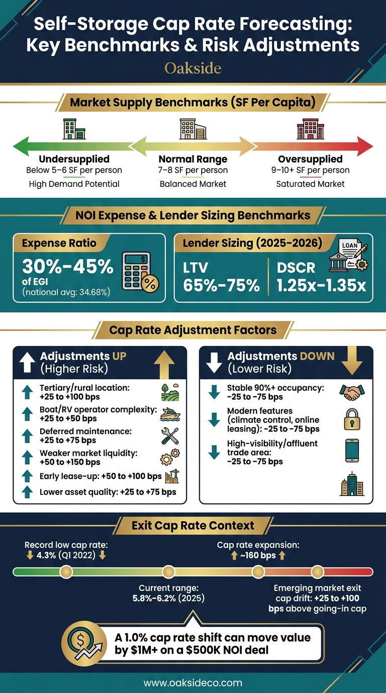
Self-Storage Cap Rate Forecasting: Key Benchmarks & Risk Adjustments
Step 1: Screen the Market and Build a Defensible Comp Set
Only screen markets that have enough demand, clear supply data, and enough deal activity to support a cap-rate range you can defend.
Map Demand, Supply, and Trade Area Boundaries
Start with the right trade area. For suburban self-storage, use a 3- to 5-mile trade area. In dense urban cores, use 1- to 3-miles. In rural or exurban markets, use 5- to 10-miles. For boat & RV storage, use 15- to 30-minute drive times instead of a basic radius.
Physical barriers matter too. A river, highway, or rail corridor can split a trade area in practice, even when the straight-line distance looks fine on a map.
When comparing self-storage vs boat & RV storage, a simple radius won’t do the job. RV and boat owners will often drive farther if the site fits their needs. That’s why drive-time analysis works better here. Add state DMV or county registration data for boats and RVs, then map distance to lakes, marinas, coastal access points, and major highway corridors. A site near a recreation corridor or a second-home market can pull demand from a 20- to 40-minute drive-time area, even in a smaller market.
After the trade area is set, track the demand drivers that move the needle:
- Household and population growth
- Net migration
- Housing turnover
- Population density
- Median household income
On the supply side, calculate existing storage square feet per capita inside the trade area and compare that figure with market norms. National self-storage supply averages about 7–8 square feet per person, but the local trade-area number matters more for underwriting. Markets below 5 to 6 SF per capita can look undersupplied. Markets above 9 to 10 SF per capita start to show oversupply risk.
Don’t stop at today’s inventory. The pipeline matters just as much. Permitted and planned projects can shift the picture fast once they open.
If the trade area shows supportable demand and supply that looks manageable, move to comp pricing. If not, stop there instead of trying to force a cap-rate range that doesn’t fit.
Select Comparable Sales and Adjust for Risk
Once you’ve mapped the trade area and sized up demand and supply, the next job is to build the comp set.
In newer markets, local sales are often too thin to pin down a cap rate by themselves. The practical move is to go broader on geography while getting stricter on asset filters. Pull recent sales from the state or region, then screen them by asset quality, product type, occupancy, and stabilization status.
If a comp comes from a stronger or more liquid market than the subject property, adjust upward. Use upward adjustments for:
- Weaker liquidity: +50 to +150 bps
- Early lease-up: +50 to +100 bps
- Lower asset quality: +25 to +75 bps
Write down the reason for each adjustment. That matters when a lender or investor starts asking hard questions. The adjusted comp set gives you the pricing floor and ceiling for the market, and that becomes the frame for the NOI cases in Step 2.
sbb-itb-09b4138
Step 2: Underwrite NOI and Set a Cap Rate Range
Once you have a defensible comp set and a market cap rate range, the next move is to turn that market range into asset-level NOI. That’s what drives pricing. Put simply, the asset’s current and projected NOI is what tells you where the deal should trade.
Start with the T-12 operating statement and rent roll. Clean up the numbers by removing seasonality, one-time repairs, and concessions like first-month-free promotions. Then compare in-place rents against current street rates to find rent upside. T-12 occupancy can also understate the asset’s actual run rate, so don’t treat it as the whole story.
For expenses, use 30%–45% of EGI as a benchmark. The national average is about 34.68%. If expenses are understated, cap rates look lower than they should and implied value gets pushed too high. That normalized NOI is the base for your scenario work.
Build Baseline, Stabilized, and Downside Cases
Don’t price from a single NOI figure. Build three cases and test each one against the market cap-rate range.
- Baseline: Current T-12 results, normalized expenses, and modest occupancy and rent gains.
- Stabilized: 90%–92% physical occupancy, market rents, and normalized staffing levels.
- Downside: 80%–82% occupancy, new-supply pressure, and higher marketing spend.
A small shift in occupancy, rent, or expenses can move value by a lot. That’s why single-point pricing can get you in trouble fast.
From there, adjust the cap rate for property-level risk.
Apply Asset-Level Basis Point Adjustments
The market comp set gives you a starting cap rate. Then you move that number up or down based on the asset in front of you. Each adjustment should be written down on its own so lenders and investment committees can follow the reasoning.
Cap rate adjustments usually move higher when the deal carries more risk. That can include a tertiary or rural location with thin buyer demand (+25–100 bps), operator complexity like boat/RV storage that needs specialized management (+25–50 bps), or deferred maintenance and functional obsolescence (+25–75 bps). If a property needs $500,000 of near-term capital work, that alone may justify a +50–75 bps adjustment.
Cap rates can also move below the market baseline. Stable 90%+ occupancy over several years, modern features like climate control and online leasing, and a high-visibility site in an affluent trade area can each support a –25–75 bps adjustment.
One thing matters here: don’t double-count risk. If lease-up risk is already reflected through lower NOI in the baseline case, don’t add a full lease-up premium again through the cap rate. That’s an easy way to distort value.
With NOI and asset risk set, test borrowing costs and exit cap assumptions next.
Step 3: Account for Debt Markets and Exit Assumptions
Factor Borrowing Costs Into Required Yield
Cap rates move with financing. In newer, less liquid storage markets, lender behavior often sets the upper limit on what buyers can pay.
Most lenders size self-storage loans to whichever is tighter: DSCR or LTV. In 2025–2026, the working range is usually 65%–75% LTV and 1.25x–1.35x DSCR. In a thin or less proven market, lenders often get stricter and underwrite below the sponsor’s pro forma occupancy and rent.
That matters because lender limits can be turned into a hard value ceiling. Say a deal has stabilized NOI of $600,000. At those loan-sizing thresholds, the market may only support a value in the $10.4 million to $10.5 million range. Then add the equity side. If investors want at least a 250–300 bps spread over their debt cost, pricing moves closer to a 7.5%–8.0% cap rate, which points to a value of about $7.5 million to $8.0 million.
Higher borrowing costs and tighter lender sizing push cap rates up and bids down. That isn’t a flaw in the model. It’s the model doing its job.
Once lender sizing sets the buy-side ceiling, the next step is simple: check whether the exit cap still makes the hold work.
Set Exit Caps Using Forward NOI, Not Trailing NOI
Apply the exit cap to forward NOI, not trailing NOI. That’s how institutional buyers tend to think about value. They price based on what the asset is likely to earn in the year after they buy it, so the exit model should follow that same logic.
In practice, use the forward NOI case you already underwrote. Project NOI through each year of the hold, then divide NOI in the year after sale by the exit cap to get the implied sale price.
For the exit cap, start with the going-in cap and add a spread for hold period length, market stabilization, and liquidity risk. In emerging storage markets, a 25–75 bps upward drift is a reasonable base case. If the market is less certain, 50–100 bps may be more fitting.
A 5-year hold with $675,000 of forward NOI and a 7.75% exit cap implies an $8.71 million sale price.
A Practical Framing for Uncertain Markets
In uncertain markets, use a range and then pressure-test it with slower rent growth and wider exit caps. The point is to build a realistic value range from well-underwritten fundamentals, then see how it holds up under debt and exit cases that could actually happen.
Self-storage cap rates expanded by roughly 160 basis points from a record-low 4.3% in Q1 2022 to about 5.8%–6.2% by 2025, driven mostly by higher interest rates. So if a model assumes cap rate compression without clear signs of market stabilization, NOI growth, and better liquidity, it will likely overstate exit value.
That risk gets sharper in newer markets. Liquidity is thinner, stabilization may still be underway, and buyers usually demand more yield for that extra uncertainty. A disciplined model keeps the exit cap flat to slightly wider in the base case and saves compression scenarios for upside cases.
Step 4: Check for Common Forecast Errors Before Finalizing Value
Once your debt and exit assumptions are in place, do one last QC pass on the comp set, NOI, and cap rate before you use any value estimate to price an acquisition, set a sale target, or back up a refinance.
Errors That Skew Storage Cap Rate Forecasts
Start with comps. If you pull in core-market comps and apply them as-is, you can understate local risk. Adjust for liquidity, demand stability, and operator quality before applying any comp to the subject asset.
Next, don’t price off trailing NOI. Trailing figures can throw off value and create a mismatch with hold-period economics. Use stabilized forward NOI as your anchor, and treat trailing NOI as a gut check.
Also, don’t use one cap rate for every asset type. A Class A climate-controlled facility, a Class C drive-up, and a boat & RV property do not carry the same risk. Your cap rate needs to match the asset’s class, climate-control mix, lease-up status, and specialty use.
National averages can help as a starting point. But they shouldn’t make the final call. Local rent trends, the supply pipeline, regional trades, and lender feedback should drive cap rate selection.
Final Validation and Conclusion
Use this last check to see whether the model still works under slower NOI growth and wider exit caps. Before you lock in value, make sure comp adjustments, forward NOI, asset-level cap rates, and exit assumptions all line up.
| Common Error | Impact on Valuation | Corrective Step |
|---|---|---|
| Misusing core-market comps | Underestimates risk; leads to overpayment | Adjust for liquidity, demand stability, and operator quality; cross-check with regional trades |
| Using trailing NOI instead of forward NOI | Misaligns with hold-period economics | Anchor to stabilized forward NOI; use trailing NOI only as a sanity check |
| Applying one cap rate across all asset types | Poor risk pricing; overvalues higher-risk assets | Define cap rate bands by class, climate control, lease-up status, and specialty type |
| Ignoring liquidity discounts for boat & RV assets | Overstates exit value; underestimates sale timing risk | Assess buyer depth and recent trades; add a quantified liquidity adjustment of 25–100 bps where warranted |
| Over-relying on national averages without local context | Imports inappropriate assumptions; misses local demand and supply shifts | Use national surveys as directional benchmarks only; prioritize local comps, rent data, and lender feedback |
FAQs
How many comps are enough in a new market?
Analyze 5 to 10 recent sales of comparable properties. Focus on deals that match the subject asset in size, property type, and occupancy so the numbers reflect the local trade area as closely as possible.
Then, for each sale, calculate the cap rate by dividing trailing 12-month net operating income by the sale price. This gives you a market-based cap rate you can use for underwriting.
Put simply:
- Find recent comps that look like the asset you’re reviewing
- Use each property’s TTM NOI ÷ sale price
- Compare the results to land on a cap rate that fits the market
If the comps aren’t close matches, the cap rate can drift and give you the wrong read on value.
When should I use forward NOI instead of trailing NOI?
Use trailing 12-month (T-12) NOI first to anchor valuation in proven property performance and current market conditions. In most deals, buyers put more weight on what the property has already produced than on projected numbers.
Then use forward, or pro forma, NOI to test future scenarios. This matters most for value-add, lease-up, or expansion deals that are priced based on stabilized performance. Build in monthly assumptions for seasonality, lease-up pace, and expected rent growth.
How much should I widen the exit cap in an emerging market?
In emerging markets, it’s smart to widen your exit cap rate by 50 to 150 basis points to account for liquidity risk and a thinner buyer pool. Supply and demand can swing more in these markets, so a conservative exit assumption helps keep your model grounded.
It also helps to stress-test your projections in 25 to 50 basis point steps, and cover at least 400 basis points around your base case. That gives you a clearer read on how the deal holds up if market conditions shift.