

If I want a solid self-storage value range, I start with recent sales, then trim the list hard. The best comp set usually comes from arm’s-length sales in the last 12–24 months, in the same submarket, with assets near 85%–95% occupancy and a similar product mix.
Here’s the short version:
- I compare deals using $/rentable sq. ft., cap rate, revenue per occupied sq. ft., and NOI per rentable sq. ft.
- I remove weak comps, like distressed sales, related-party deals, and lease-up assets under 80% occupancy
- I keep climate-controlled, drive-up, and boat/RV income separate so the math doesn’t get distorted
- I adjust for time, location, and asset quality
- Then I check value using two methods at once: $/sq. ft. and cap rate
- Last, I stress-test changes in occupancy, NOI, and cap rate, because small shifts can move value by hundreds of thousands of dollars
A few numbers show why this matters. A $1.00 change in rent on a 60,000-sq.-ft. facility can add about $60,000 in annual revenue. At a 6.0% cap rate, that can mean about $1,000,000 in value. And if a property has $600,000 in NOI, moving the cap rate from 6.25% to 5.75% changes value from about $9,600,000 to $10,435,000.
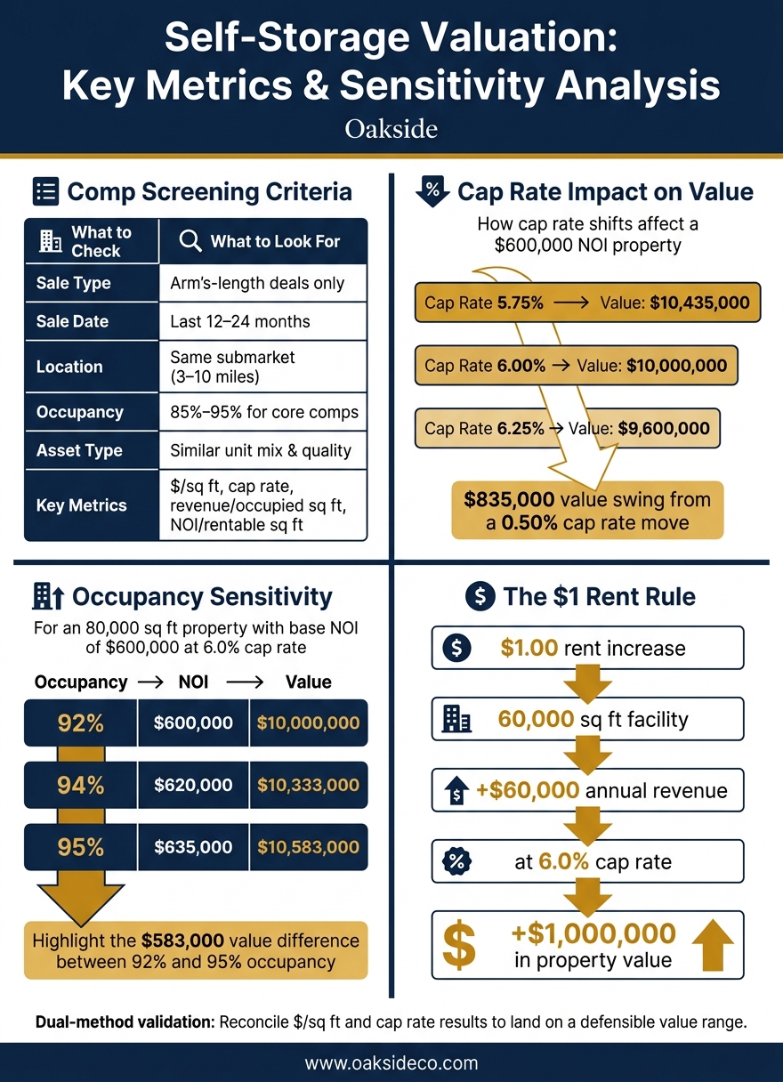
Self-Storage Valuation: Key Metrics & Sensitivity Analysis
Quick comparison
| What I check | What I’m looking for | Why it matters |
|---|---|---|
| Sale type | Arm’s-length deal | Filters out prices that don’t reflect the open market |
| Sale date | Last 12–24 months (a standard window for exit planning) | Keeps pricing tied to today’s market |
| Location | Same submarket, often within 3–10 miles | Rent, taxes, and supply can shift a lot inside one metro |
| Occupancy | Usually 85%–95% for core comps | Helps separate stabilized assets from lease-up deals |
| Asset type | Similar unit mix and quality | A Class A climate-controlled site is not the same as an older drive-up asset |
| Key metrics | $/sq. ft., cap rate, revenue/occupied sq. ft., NOI/rentable sq. ft. | Shows price, income, and efficiency on the same basis |
| Final check | Reconcile $/sq. ft. and cap rate results | Helps me land on a tighter value range |
The main point: I don’t use nearby sales just because they’re nearby. I use the sales that match the subject on market, timing, and income profile, then I turn that data into a value range I can support.
sbb-itb-09b4138
2. How to Build a Reliable Comp Set
2.1 Screen for Geography, Timing, and Stabilization
Start tight on geography. A sale in the same submarket, like North Dallas instead of the full Dallas–Fort Worth metro, is often far more useful than a sale from another market. Why? Because rent levels, property taxes, and new supply can change a lot even within one MSA.
In dense coastal markets, a 3–5 mile trade area often makes sense. In suburban or rural areas, 5–10 miles is a better place to start.
Use the most recent arm’s-length sales you can find. If you’re looking at older deals, adjust them for market movement so you’re not mixing past pricing with today’s market.
For stabilization, stick with facilities that have stabilized occupancy and steady rent and occupancy trends. Properties below 80% occupancy are often still in lease-up, so they should sit in a separate bucket.
A practical way to do this is simple:
- Pull 15–25 sales that fit broad geography and timing filters
- Cut that list down to 5–10 core comps
- Remove non-arm’s-length deals, distressed sales, and clear outliers
That narrower set usually gives you something you can work with instead of a messy pile of half-relevant transactions.
2.2 Match the Right Property Characteristics
Once geography and timing are in place, match the physical product. Drive-up, climate-controlled, and mixed assets do not trade the same way, so compare like with like.
Then go one layer deeper. Look at rentable square footage, unit mix, construction quality, visibility, and age. A modern multi-story Class A facility with elevator access and advanced gate security is not a direct comp for a single-story metal-building Class B asset from the 1990s. That’s apples to oranges.
When the comps are materially different, split them into categories and apply a modest adjustment for quality gaps. That keeps the set cleaner and stops one oddball property from skewing the read.
Also, underwrite the boat/RV piece on its own. Outdoor and covered RV/boat spaces tend to move more with seasonality and local income levels. On top of that, many institutional buyers use separate return assumptions for that income stream.
2.3 How to Clean and Normalize Incomplete Comp Data
Even strong comp sets often have holes. Missing fields are normal.
If NOI isn’t disclosed, start with the sale price and rentable square feet. From there, estimate NOI using regional benchmarks. For stabilized suburban non-climate facilities, a fair starting range is $3.50–$4.50 NOI per square foot. Climate-controlled urban assets usually run higher.
Next, divide the estimated NOI by the sale price to get an implied cap rate. Then sanity-check that number against a smaller set of fully documented transactions. That extra check helps you see whether your estimate is in the right zone.
When NOI figures are available, clean them with care. Strip out nonrecurring income and expenses such as event parking, bulk rentals, insurance settlements, roof work, and one-time legal costs. Standardize management fees to market levels. And make sure you’re using a trailing twelve months (TTM) figure, not a partial-year snapshot.
The point is to get comparable NOI across every facility.
Once the set is cleaned, compare cap rate, occupancy, and revenue per square foot on the same basis.
3. Key Metrics That Drive Self-Storage Value
Once the comp set is normalized, the next step is simple: use cap rate, occupancy, and per-square-foot metrics to tell the difference between an actual pricing gap and a plain asset-quality gap, a common area where sellers get valuations wrong.
That matters because two sales can look similar on the surface and still belong in very different risk buckets.
3.1 Cap Rate and NOI
NOI is property-level income after operating expenses and before debt service, taxes, and depreciation. Cap rate is NOI divided by price.
In the self-storage space, cap rates often land in the 5%–8% range, with movement based on market type, asset quality, and stabilization status. That range gives you a practical way to sort comps. Group them by market, quality, and where they sit in the lease-up or stabilization cycle.
A newer facility in a strong growth submarket will usually trade at a tighter cap rate than an older property in a slower area. That’s normal. The problem starts when you mix primary-market trades with secondary-market sales, or lump together assets with very different risk levels. At that point, the blended figure stops telling you much.
Cap rate gives you the pricing frame. Occupancy and per-square-foot output help show whether that pricing holds up.
3.2 Physical Occupancy vs. Economic Occupancy
Physical occupancy tells you how much space is rented. Economic occupancy tells you how much income is actually collected after concessions and bad debt.
Looking at both side by side can show whether weak collections are being hidden by move-in specials, delinquency, or an asset still in lease-up.
Say your subject property is sitting at 82% physical occupancy, while nearby stabilized comps are at 92%–95%. That doesn’t mean the subject is stuck there for good. In many cases, it makes more sense to underwrite to a reasonable stabilized level and account for the value tied to closing that gap.
That adjustment should match the facts on the ground, including:
- Lease-up stage
- Market demand
- Unit mix
- Pricing strategy
The point isn’t to force the subject to look like the comps. It’s to compare them fairly.
3.3 Revenue and NOI Per Square Foot
These ratios help you compare pricing power and operating efficiency across properties that aren’t the same size. Revenue per occupied square foot shows how well the facility monetizes rented space. NOI per rentable square foot shows operating efficiency across the full asset.
If the subject property is producing much less revenue per square foot than nearby stabilized peers, that gap may support a downward valuation adjustment. Or it may point to a pricing or management opportunity that should be underwritten on its own.
One caution here: keep climate-controlled, non-climate-controlled, and boat/RV areas separate when you run these ratios. If you blend them together, the averages can get warped fast, and a mixed asset can appear stronger or weaker than it is. Boat/RV income should stay separate because it doesn’t behave like standard storage revenue.
Those normalized figures then feed into time, location, and asset-quality adjustments in the next step.
4. How to Convert Comparable Data into a Value Range
Once you’ve cleaned up the comp set, those numbers turn into pricing inputs. The goal is simple: use $/rentable sq ft and cap rate together, then reconcile where they overlap into one value range.
4.1 Adjust Comps for Time, Location, and Asset Differences
Before you apply any comp to the subject property, it has to reflect today’s market, not the market on the day it sold.
Time adjustments come first. Older sales need to be trended forward because cap rates and pricing moved in a material way from 2022 to 2025.
Location adjustments come next. Look at submarkets based on demand, supply, rent levels, and visibility. If a comp is in a stronger submarket, its $/sq ft should be adjusted downward, or its implied cap rate should be adjusted upward, before you use it for a weaker location. Typical adjustment bands run 5%–20% on $/sq ft and 25–75 basis points on cap rate, depending on how far apart the submarkets are.
Asset-level differences finish the process. Climate-control mix, physical condition, security features, unit access type, and management quality all shape achievable NOI per sq ft. A recently renovated facility with modern gate access and professional management will usually trade at a tighter cap and a higher $/sq ft than an older property with deferred maintenance, even in the same ZIP code. Document each adjustment as a range so the final value has support behind it.
After that, convert the adjusted comps into value using both pricing methods.
4.2 Derive Value Using $/Square Foot and Cap Rate Side by Side
With adjusted comps in hand, run two methods in parallel and compare the results.
The $/rentable sq ft method applies the adjusted comp range straight to the subject’s total rentable area. If adjusted comps point to $110–$130 per rentable sq ft and the subject has 75,000 rentable sq ft, the indicated value range is $8,250,000–$9,750,000.
The cap rate method uses stabilized NOI divided by the comp-derived cap rate range to produce a second value indication. For example, if stabilized NOI is projected at $575,000 and the market cap rate range is 5.75%–6.25%, the implied value range is about $9,200,000–$10,000,000.
A practical comp table should include:
- Sale date
- Price
- Size
- $/sq ft
- NOI
- Cap rate
- Occupancy
- Any boat/RV income split
That makes it much easier to see which comps are moving the indicated value and why.
Use the overlap between the two methods as the main value range. If they drift apart too much, dig into the reason. In most cases, that points to a comp that needs a heavier adjustment or a stabilized NOI estimate that’s too aggressive.
Then stress-test the range by changing occupancy, cap rate, and any boat/RV income assumptions.
4.3 Test Sensitivity for Occupancy, Rates, and Boat/RV Components
A single-point value can fall apart fast. Small shifts in occupancy or cap rate can move value in a meaningful way, so sensitivity testing matters before you show a range to investors or lenders.
Take a subject property with 80,000 rentable sq ft and a base-case stabilized NOI of $600,000 at 92% economic occupancy. At a 6.0% cap rate, that implies a value of $10,000,000. Push occupancy to 94% and NOI rises to about $620,000. Value moves to about $10,333,000. At 95%, NOI reaches around $635,000 and value gets close to $10,583,000.
Cap rate changes can hit just as hard. At 5.75%, the same $600,000 NOI implies $10,435,000. At 6.25%, it falls to $9,600,000.
For mixed self-storage and boat/RV assets, value the storage income and boat/RV income separately, then add the indications together, or apply one blended cap only after you’ve documented the split.
5. Conclusion: Using Comparables as Part of a Disciplined Advisory Process
Once you’ve turned comps into a value range, the last step is simple: check whether the market data and the property’s operating results still support the same answer. Sound valuation starts with comps, normalized NOI, and current market evidence. When comps and operating performance line up, the value range is easier to defend.
That check needs to go beyond the subject property’s current occupancy. One of the most common mistakes is looking only at trailing occupancy and ignoring the three-mile trade area of competing facilities. Supply in a submarket can change fast. Asking rates can also point you in the wrong direction because new customers are often signed at promotional rates. That creates a gap between in-place rent and current market rates. Using RevPAF as a comp-validation tool helps combine rate and occupancy into one metric that stands up across the comp set.
Ancillary income matters too. Items like tenant protection plans can materially change NOI and the comp-adjusted price. Condition and maintenance history also deserve a close look, since both can shift value.
The main idea is to stay tied to current market evidence. Use current cap rates, market-specific variables, and normalized comps to bridge buyer and seller expectations. Targeted pre-sale improvements can help, but they don’t replace a market-based valuation. That discipline leads to a value opinion buyers can defend.
FAQs
How many comps are enough?
For a reliable self-storage valuation, look at 5 to 10 recent sales of similar properties. The best comps are the ones that line up closely with your facility in size, type, and occupancy, so you’re comparing apples to apples.
Next, divide each property’s trailing 12-month net operating income by its sale price. That gives you a market-based cap rate to use in your valuation.
When should lease-up assets be excluded?
Exclude lease-up assets from stable market comparables until they reach stabilization, which is usually 85% to 90% occupancy.
Before that point, they can skew valuation metrics. Why? They come with a different risk profile, higher vacancy, and need separate underwriting for absorption.
For a cleaner analysis, compare stabilized assets with properties at a similar operating stage.
Which metric matters most for value?
Net Operating Income (NOI) is the key metric in self-storage valuation. As Nolen Masserman, Managing Director at Oakside, notes, these assets trade on cap rates applied to stabilized NOI, not gross revenue or facility size.
That matters because value is calculated by dividing NOI by the cap rate. So even small shifts in income or expenses can have a big effect on valuation.