
Break-even occupancy is the minimum percentage of rented units a self-storage facility needs to cover all operating expenses and loan payments, leaving no profit or loss. If occupancy drops below this level, the business operates at a loss. This metric is vital for assessing financial stability and understanding how much room exists before losses occur.
Key Points:
- Break-even occupancy differs from physical or economic occupancy. It focuses solely on financial sufficiency.
- Facilities with debt typically need 60–65% occupancy to break even, while debt-free properties require only 30–35%.
- Lenders often require a Debt Service Coverage Ratio (DSCR) between 1.20x and 1.35x, ensuring income exceeds break-even levels.
- Operating expenses (OPEX), debt service, and potential gross income (PGI) are essential inputs for calculating break-even occupancy.
Quick Example:
- A facility with $153,800 in annual costs and $216,000 in PGI has a break-even economic occupancy of 71.2%.
This metric helps operators and investors evaluate risk, adjust strategies, and navigate challenges like competition or market downturns.
Key Metrics Needed for Break-Even Calculations
To calculate break-even occupancy, you need three key inputs: operating expenses (OPEX), debt service, and potential gross income (PGI). These metrics are the foundation for determining when a facility becomes financially self-sufficient. Accurate data for each is essential to ensure a reliable analysis.
Operating Expenses (OPEX)
Operating expenses include all the costs required to run the facility daily. This covers property taxes, insurance, payroll, utilities, marketing, repairs, and management fees. These expenses represent the baseline revenue needed before addressing debt or generating profit.
One common pitfall among investors is relying on the seller’s expense data without adjustment. Many owner-operators exclude management fees or understate payroll costs (sometimes paying themselves nothing). If you don’t normalize these figures, Net Operating Income can be inflated by 10–15%. The table below outlines typical expense ranges, including management fees:
| Expense Category | Typical Range (% of EGI) |
|---|---|
| Property Taxes | 8% – 15% |
| Payroll | 8% – 15% |
| Management Fee | 5% – 6% |
| Utilities | 3% – 8% |
| Marketing & Advertising | 2% – 5% |
| Repairs & Maintenance | 2% – 5% |
| Insurance | 2% – 4% |
Another factor to watch is property tax reassessment risk. In many areas, a sale can trigger a reassessment that increases property taxes significantly. Since taxes typically account for 8–15% of Effective Gross Income (EGI), this single expense can have a major impact on your break-even analysis. Performing a sensitivity analysis can help you understand how these fluctuations affect your bottom line.
Once OPEX is accounted for, the next step is to evaluate the role of debt service.
Debt Service
Debt service includes the total annual cost of your loan, combining both principal and interest payments. For properties with financing, this is often the largest expense, requiring occupancy in the low-to-mid 60% range to break even. In contrast, debt-free properties typically need only 30–35% occupancy to cover costs.
The terms of your loan heavily influence this figure. A higher loan-to-value (LTV) ratio results in a larger loan balance, increasing annual payments. Similarly, higher interest rates amplify these costs. To calculate debt service accurately, you’ll need three key pieces of information: the total loan amount, the annual interest rate, and the amortization period.
With debt service addressed, the final piece in the break-even framework is potential gross income.
Potential Gross Income (PGI)
PGI represents the maximum revenue your facility could generate if every unit were rented at full market rates, with no vacancies, concessions, or bad debt. It functions as the denominator in the break-even formula – the higher the PGI, the lower the occupancy percentage required to cover fixed costs.
It’s important to distinguish between street rates (advertised prices) and stabilized market rents. Street rates fluctuate daily based on inventory and are often discounted to attract new tenants. For underwriting purposes, PGI should reflect the median achievable rent in the area under stable conditions, not temporary promotional rates. Always compare advertised rates with the actual rent roll to see what tenants are actually paying versus what’s being advertised.
Additionally, ancillary income – such as late fees and tenant insurance – can add an extra 3–8% to revenue. While not part of PGI, it’s worth considering separately when analyzing the overall income potential of the facility.
sbb-itb-09b4138
Formulas for Calculating Break-Even Occupancy
Once you’ve gathered your OPEX, debt service, and PGI figures, it’s time to dive into the calculations. There are three key formulas to follow, each building on the previous one.
Break-Even Revenue
The first step is calculating your break-even revenue:
Break-Even Revenue = Operating Expenses + Debt Service
This figure tells you the minimum annual income your facility needs to stay afloat – not to turn a profit, but simply to cover costs. For instance, if your normalized OPEX is $59,000 annually and your debt service totals $94,800, your break-even revenue is $153,800. Falling short of this amount means operating at a loss.
It’s worth noting that lenders often require replacement reserves of around $0.25 per rentable square foot per year. Be sure to include these reserves in your OPEX before running the calculation.
Economic Occupancy Formula
Once you know your break-even revenue, the next step is to calculate economic occupancy. This is done by dividing your break-even revenue by your PGI:
Break-Even Economic Occupancy = Break-Even Revenue ÷ PGI
Using the earlier example, with $153,800 in fixed costs and a PGI of $216,000, the break-even economic occupancy is 71.2%. This means your facility must generate revenue equal to at least 71.2% of its PGI to cover costs.
Economic occupancy is a more nuanced metric because it accounts for factors like concessions, free-month promotions, and delinquent payments – things that can reduce actual revenue even when units are physically occupied. In practice, economic occupancy tends to run 3% to 8% lower than physical occupancy at most facilities.
Physical Occupancy Formulas
Physical occupancy can be calculated in two ways, depending on your facility’s unit mix:
| Method | Formula | Best Used When |
|---|---|---|
| Unit-Based | (Occupied Units ÷ Total Units) × 100 | All units are similar in size |
| Square-Footage-Based | (Occupied Sq. Ft. ÷ Total Rentable Sq. Ft.) × 100 | Unit mix varies significantly |
For facilities with a mix of unit sizes – like 5×5 units alongside 10×30 ones – the square-footage method provides a clearer picture of actual usage. For example, a facility might show 90% unit occupancy but still have its largest, highest-revenue units sitting empty, which the unit-based formula wouldn’t reveal.
While physical occupancy is a useful operational metric, it’s the economic occupancy figure that carries more weight for underwriting and investment decisions. High physical occupancy doesn’t mean much if significant discounts or unpaid rents are dragging down revenue. These formulas lay the groundwork for the more detailed break-even analysis covered in the next section.
Step-by-Step Process to Calculate Break-Even Occupancy
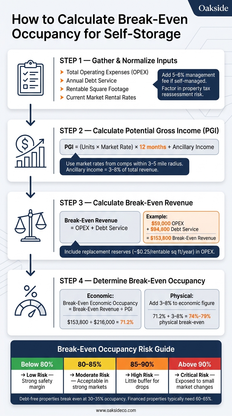
How to Calculate Break-Even Occupancy for Self-Storage
Let’s break down the process of calculating break-even occupancy using practical steps and clear formulas.
Gathering and Normalizing Inputs
Start by collecting accurate and detailed data. The key inputs include your total operating expenses (OPEX), annual debt service, rentable square footage, and current market rental rates for each unit type.
Normalization is a critical step that operators often overlook, especially when analyzing potential acquisitions. Two adjustments are particularly important:
- If the property is self-managed, include a 5% to 6% management fee, even if no one is currently being paid for this role. This adjustment reflects the actual cost of professional management and ensures your analysis is defensible.
- Factor in the risk of property tax reassessment. Ignoring this can make a deal seem more profitable than it truly is, especially when running monthly models that account for seasonal revenue changes.
These normalized inputs are essential for calculating the Potential Gross Income (PGI).
Calculating Potential Gross Income
Once your expenses are normalized, the next step is determining your Potential Gross Income (PGI) – the maximum revenue your facility could generate at 100% occupancy with full market rates.
Instead of relying on the seller’s current rents (which might be outdated or include discounts), use market rates from a comp survey within a 3–5 mile radius. The table below outlines how PGI is calculated by component:
| PGI Component | Data Needed | Calculation |
|---|---|---|
| Base Rental PGI | Unit mix (quantity × size) + market rate | (Units × Market Rate) × 12 months |
| Ancillary PGI | Protection plans, retail, late fees | Estimated annual total at full use |
| Total PGI | Sum of all potential revenue | Base Rental PGI + Ancillary PGI |
Don’t forget to include ancillary income streams, such as tenant protection plans, retail sales (locks, boxes), and late fees. In well-run facilities, these can make up 3% to 8% of total revenue.
Determining Break-Even Occupancy
With both PGI and break-even revenue established, you can now calculate the occupancy level needed to cover costs. Divide the break-even revenue by the PGI to find the economic break-even occupancy.
Here’s an example:
- A 150-unit facility charges $120 per unit per month, resulting in an annual PGI of $216,000.
- If normalized OPEX is $59,000 and annual debt service is $94,800, the break-even revenue is $153,800.
- Economic break-even occupancy is calculated as $153,800 ÷ $216,000, which equals 71.2%.
To convert this to a physical break-even occupancy, you’ll need to adjust for factors like concessions, free-move-in promotions, and bad debt. Add 3% to 8% to the economic figure, placing the physical break-even occupancy between 74% and 79% in this example.
A good practice is to run this calculation monthly to account for seasonal variations in revenue. For instance, self-storage demand typically peaks between May and September, and relying on a single annual figure might obscure periods when the property falls below break-even.
Using Break-Even Occupancy for Decision-Making
Operational Insights
Break-even occupancy serves as a practical tool for managing operations. For example, if physical occupancy falls below 85%, it might be time to adjust strategies – like lowering street rates, offering promotions, or reevaluating underperforming unit types. A 10×5 climate-controlled unit might require a different approach compared to a 10×20 drive-up unit.
Another key metric to monitor is Revenue Per Available Square Foot (RevPAF), which is calculated by dividing annual rental revenue by total rentable square footage. Comparing your RevPAF to other facilities within a 3–5 mile radius can reveal whether pricing or management practices need adjustment. If your RevPAF is trailing behind local competitors, operational changes may be necessary before considering rent increases.
Cost-cutting measures, such as automating payroll with kiosks or online booking systems, can also make a difference. Payroll costs, which typically account for about 15% of Effective Gross Income (EGI), can potentially drop to around 8% with automation. This reduces the revenue required to cover expenses, ultimately lowering the break-even point.
While these operational adjustments are crucial for day-to-day management, break-even occupancy also plays a critical role in broader financial decisions.
Underwriting and Investment Analysis
In underwriting, break-even occupancy acts as a stress test to assess a property’s long-term financial health. Ideally, the break-even occupancy level should sit well below the market’s stabilized occupancy range, which typically falls between 85% and 92%. If the break-even point is significantly lower than this range, the property has a safety cushion. On the other hand, a break-even level that’s too close to market occupancy signals potential risk.
Leverage greatly impacts this equation, as debt service costs often drive break-even thresholds higher. For acquisitions or development projects with significant financing, it’s essential to evaluate the Debt Service Coverage Ratio (DSCR) over multiple years – not just at stabilization. This ensures that Net Operating Income (NOI) consistently exceeds debt payments by the required margin set by lenders.
Another factor to consider is property tax reassessment, which can occur after a purchase. Taxes might be recalculated based on the new sale price, potentially increasing by 2× to 7×. This can significantly raise the break-even occupancy requirement. To avoid surprises, engaging with the local tax assessor before closing can help manage potential cost increases in the first year.
The Role of Advisory Firms
Accurate break-even analysis depends on reliable data and a deep understanding of local market dynamics. Firms like Oakside Co specialize in working with institutional self-storage owners and investors to create detailed, market-specific break-even analyses. Their process includes normalizing management fees, accounting for potential tax reassessments, and benchmarking RevPAF against competitive properties. This thorough approach ensures that decisions – whether for acquisitions, dispositions, or refinancing – are based on solid, defensible data rather than overly optimistic projections.
Nolen Masserman, Managing Director at Oakside, highlights the importance of reliable inputs for break-even analysis: “Standardized expenses, verified rent rolls, and robust local comparables are essential to any credible underwriting analysis.”
Conclusion: Key Takeaways on Break-Even Occupancy
Break-even occupancy pinpoints the revenue a facility needs to cover its costs and highlights how much breathing room exists before losses occur. For example, a facility with a break-even point at 65% occupancy but operating at 88% has a comfortable cushion. On the flip side, a facility breaking even at 85% has little room for error, especially when month-to-month leases can cause revenue fluctuations of 10%–15% per quarter. This metric is essential for shaping both operational strategies and financial decisions.
Debt plays a big role in determining break-even occupancy levels. Facilities without leverage often break even in the low-to-mid 30% occupancy range. However, financed properties typically need 60%–65% occupancy to stay afloat. Before taking on new loans, it’s vital to stress-test how different financing options could impact your break-even point, particularly when compared to historical market lows in your area.
Operationally, economic occupancy is the key figure to watch. While physical occupancy shows how many units are filled, economic occupancy reflects actual revenue after accounting for concessions and bad debt. A gap of just 3%–8% can be the difference between staying above or falling below break-even.
| Break-Even Occupancy Rate | Risk Level | What It Means |
|---|---|---|
| Below 80% | Low | Offers a strong safety margin for stabilized properties |
| 80%–85% | Moderate | Generally acceptable in strong markets |
| 85%–90% | High | Leaves little buffer for occupancy drops |
| Above 90% | Critical | Highly exposed to even small market changes |
As discussed earlier, tools like RevPAF and monthly cash flow models are invaluable for monitoring break-even occupancy. Together, they help highlight a facility’s operational resilience and provide a clear picture of financial health. By consistently tracking these metrics, you can better manage risks and make informed decisions, tying together all the strategies and insights shared throughout this guide.
FAQs
Should I use economic or physical occupancy for break-even?
Economic occupancy stands out as a stronger metric for break-even analysis because it captures the actual revenue generated, factoring in discounts and concessions. This approach offers a more precise comparison to gross potential revenue, giving a clearer picture of financial performance.
What expenses are most often missed in break-even math?
When calculating break-even points, some expenses often slip through the cracks. For instance, property taxes can unexpectedly spike after a reassessment, especially following a property sale. This can have a notable impact on your calculations if not accounted for.
Another area to watch is operational costs – things like insurance and utilities. These expenses can climb quicker than anticipated, depending on market conditions or other external factors. If your models don’t account for these potential increases or aren’t stress-tested, they could lead to inaccurate projections.
How does financing change my break-even occupancy?
Financing increases the break-even occupancy rate for self-storage facilities because properties with debt require higher occupancy – usually in the low to mid-60% range – to cover both operating expenses and debt payments. On the other hand, properties without financing often break even at much lower occupancy levels, typically in the low to mid-30% range. According to Cameron Vale, President at Oakside, factors like the debt service coverage ratio (DSCR) are key in shaping these occupancy thresholds.