Self-storage follows a clear yearly pattern: leasing is strongest from late spring through summer, weakest in winter, and occupancy often peaks after leasing slows. If I want to read a market the right way, I can’t look at occupancy alone. I need to check street rates, concessions, move-in pace, and revenue quality at the same time.
Here’s the short version:
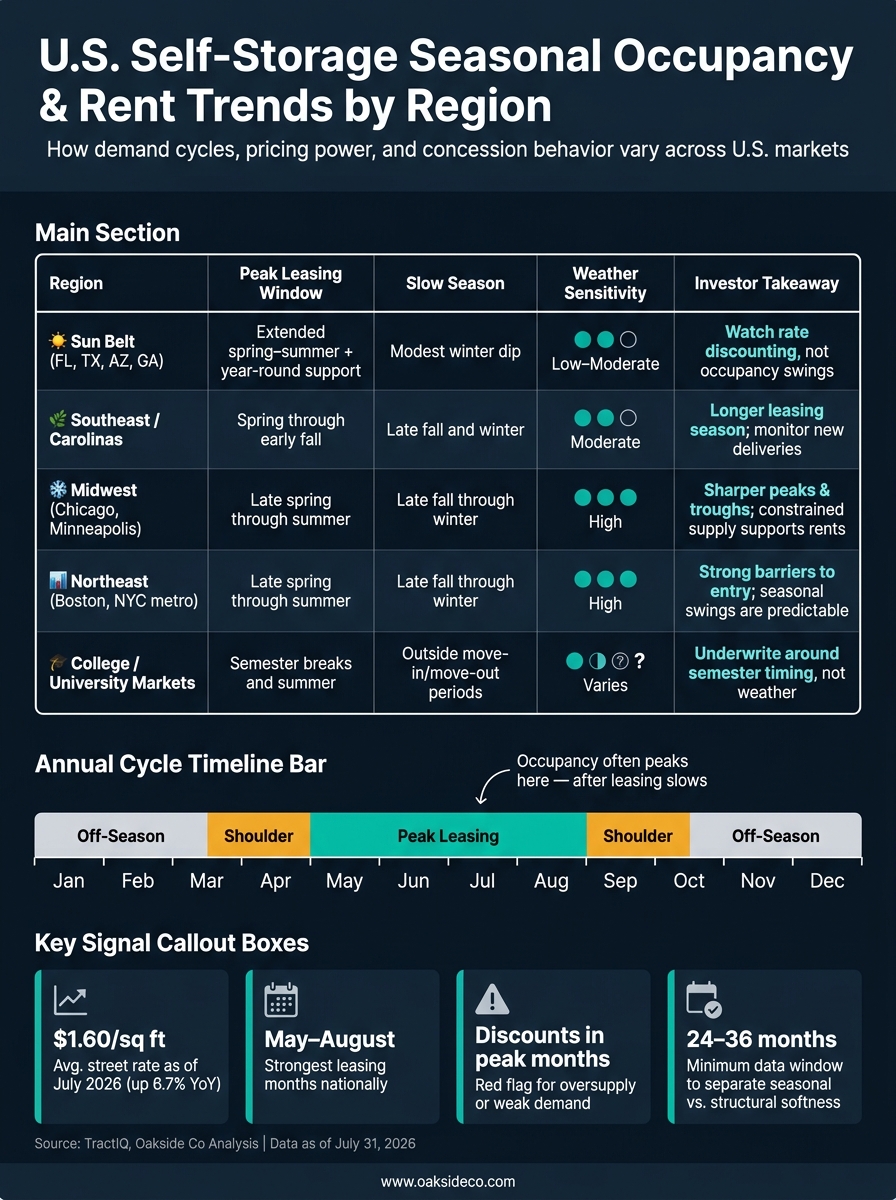
- Peak leasing usually runs from May to August
- January and February are often the slowest months
- Occupancy can stay high into fall even when demand is cooling
- A 90%+ occupied property can still have weak rent performance
- Seasonality looks different in the Sun Belt, Midwest, Northeast, and student-heavy markets
- As of July 31, 2026, average street rates were $1.60 per square foot, up 6.7% year over year
- I should use 24 to 36 months of monthly data before deciding whether softness is seasonal or a deeper demand problem
A simple way to read the market: if rates firm up and discounts fade during peak season, demand is likely healthy. If discounts stay heavy into spring and summer and rates stay below prior peaks, that often points to oversupply or weak demand.
| What I’m Watching | What It Usually Tells Me |
|---|---|
| Physical occupancy | How full the property is |
| Economic occupancy | How much of that occupancy is turning into rent |
| Street rates | Current pricing power |
| Concessions | Whether leasing is being supported by discounts |
| Net rentals and churn | Whether demand is building or slipping |
This article breaks down how that cycle works, how it shifts by region, and how I can use it when looking at pricing, budgeting, and deal timing.
2. The Typical Annual Occupancy Cycle
Self-storage tends to follow a pretty clear annual rhythm. Move-ins usually pick up from March through August. Physical occupancy often tops out in August or September. Then new rentals slow down the most from December through February.
That pattern shows up most clearly in markets where moving activity tracks with weather and housing turnover.
Peak leasing months and what drives demand
Late spring and summer bring a cluster of move-related events, and that pushes demand higher. Residential lease expirations, home sales, military Permanent Change of Station cycles, and college move-outs all stack up around the same time. Add warm weather to the mix, and moving gets easier, which adds even more lift to seasonal demand.
Slower periods and how softness shows up in the data
By November, leasing starts to cool. Promotions become more common, and street rates often level off or dip for unit sizes with a lot of competition.
Why occupancy often lags leasing momentum
Occupancy usually trails leasing momentum for a simple reason: existing tenants don’t leave the moment new move-ins slow down.
Household tenants, small-business tenants, and people renting because of life events often keep their units for months or even years. So even when new leasing cools, occupancy can stay high well into the fall and winter. In many cases, rent growth and concession trends shift before occupancy does.
The overall timing is pretty steady across the country, but climate and migration patterns can change how sharply the pattern shows up from one region to another.
sbb-itb-09b4138
3. Regional Demand Shifts Across U.S. Markets
U.S. Self-Storage Seasonal Occupancy & Rent Trends by Region
National seasonality can hide what’s happening on the ground. Each local market has its own rhythm, shaped by climate, migration, housing turnover, university calendars, tourism, and local economic conditions. That matters because the same drop in occupancy can be normal in one city and a red flag in another.
Sun Belt, coastal, and migration-driven markets
Tampa, Phoenix, Atlanta, and many markets across Florida and the Southeast tend to see steadier demand through the year. In-migration, retiree moves, tourism, and milder weather help smooth out the usual seasonal swings. In coastal and vacation-heavy areas, snowbird demand can also support fall and winter occupancy, which softens the usual cold-season slowdown.
Housing stock plays a part too. Homes in the Northeast and Midwest are more likely to have basements, while homes in Texas and Florida often do not. That pushes more households in Sun Belt markets to rely on self-storage.
But there’s a catch. The pandemic-era building surge changed the setup. A lot of new supply hit these markets right as migration cooled after 2023, leaving many Sun Belt submarkets with too much space to fill. So now, seasonality often shows up less in occupancy swings and more in pricing. During slower months, operators tend to use deeper concessions. Then in late spring and summer, they push rates harder.
Midwest and Northeast winter-sensitive markets
Chicago, Boston, and Minneapolis usually show a more obvious peak-and-trough pattern. Cold weather, snow, and tough moving conditions slow move-ins from late fall through winter. Then spring hits, and leasing activity tends to snap back fast, often with a sharper ramp than many Sun Belt markets get.
New supply has been held back more in these regions because of higher construction costs and tighter regulation, which has eased some competitive pressure. Occupancy and rents still move up and down more sharply across the year, with a clear spring pickup and winter softness, but pricing pressure from new competition is lower.
Region-by-region seasonality comparison
Student-heavy markets follow a different clock. Their demand is tied more to the academic calendar than the weather.
| Region | Typical Peak Leasing Window | Slow Season | Weather Sensitivity | Key Demand Drivers | Investor Takeaway |
|---|---|---|---|---|---|
| Sun Belt (FL, TX, AZ, GA) | Extended spring-to-summer, year-round support | Modest winter dip | Low to moderate | In-migration, retirees, no-basement housing | Watch rate discounting more than occupancy swings; supply levels matter most |
| Southeast / Carolinas | Spring through early fall | Late fall and winter | Moderate | Household formation, migration, military PCS | Longer leasing season; monitor new deliveries closely |
| Midwest (Chicago, Minneapolis) | Late spring through summer | Late fall through winter | High | Housing turnover, spring resets, limited supply | Sharper peaks and troughs; constrained supply supports rents |
| Northeast (Boston, NYC metro) | Late spring through summer | Late fall through winter | High | Dense households, constrained development, high barriers to entry | Strong barriers to entry; seasonal swings are predictable and manageable |
| College/University markets (all regions) | Semester breaks and summer | Outside move-in/move-out periods | Varies | Academic calendar, student moves | Underwrite around semester timing, not weather alone |
The next step is to read occupancy, rents, and concessions together to separate seasonal noise from structural weakness.
4. How to Read Rent and Occupancy Data for Market Timing
Reading occupancy and street-rate moves together
After you map regional seasonality, the next step is figuring out what’s normal calendar-driven movement and what points to weaker demand. No single metric can do that on its own. You need to read occupancy, street rates, and move-in pace together.
Street rates are the advertised prices for new tenants. In-place rents are what current tenants are paying. The spread between the two tells you a lot about pricing power. If a facility is sitting above 90% occupancy but street rates keep drifting down, that often means the operator is protecting occupancy by giving up rate growth. That’s why occupancy by itself can paint the wrong picture if you don’t compare it with street-rate direction and concession activity.
A better pattern looks like this: occupancy is healthy, even if not fully stabilized, while street rates are moving up and discounting is getting lighter. That usually signals demand is building and pricing power is getting better. As of July 31, 2026, TractIQ reported an average monthly street rate of $1.60 per square foot, up 6.7% year over year.
Normal seasonality versus structural weakness: key signals
The hard part in self-storage is telling the difference between a normal seasonal dip and a real demand issue. Winter softness is normal. Softness that drags into late spring or summer usually is not.
A few patterns make that distinction easier:
- Discounts that don’t taper off in peak months. Promotions like “50% off the first three months” are common in the off-season. If they’re still showing up during peak leasing months, that’s a red flag.
- Weak leasing during the spring and summer window. If move-in volume doesn’t bounce back during the strongest part of the year, demand may be under pressure.
- Street rates that remain below prior-year peaks. Winter rate cuts are normal. But if rates still haven’t recovered when demand should be strongest, pricing power likely hasn’t improved.
- High churn outside normal move-out periods. Steady turnover can point to local oversupply or weak retention.
Context still matters. A Sun Belt submarket with a lot of new supply may show rent pressure first, while a slower-growth Midwest market may hold occupancy longer before pricing starts to slip.
Seasonal phase and operating signals: comparison table
Use the table below to separate normal seasonal behavior from structural stress.
| Seasonal Phase | Move-In Pace | Occupancy Trend | Street-Rate Behavior | Discount Usage | Revenue-Management Response |
|---|---|---|---|---|---|
| Peak Season (late spring through early fall) | High | Rising or stable at high levels | Increasing; testing rate ceilings | Minimal; promotions pulled back | Tightening pricing, restricting concessions, pushing high-demand unit sizes |
| Shoulder Season (spring and fall transitions) | Moderate, building or tapering | Holding steady | Flat to modestly rising or easing | Selective; used to maintain move-in flow | Gradual adjustments; monitoring occupancy closely |
| Off-Season (winter) | Low to moderate | Flat or slight dip | Flat to slightly reduced | Targeted promotions to protect occupancy | Occupancy-protection mode; avoiding deep discounting |
| Structural Weakness (any season) | Fails to recover in peak months | Declining across multiple phases | Remains below prior-year peaks | Heavy discounting persists through peak months | Consistently defensive; rate increases not sticking |
Structural weakness is the warning sign that matters most. If a property is putting up this kind of performance during months that should look more like peak season, the problem probably won’t disappear just because the calendar flips.
For underwriting and acquisition work, the practical takeaway is simple: don’t annualize peak-season performance without adjusting for seasonality, and don’t treat winter softness as structural until you check whether the same thing happened in the prior spring. What matters most is the direction of change – and whether it holds – for 24 to 36 months, not any single month’s print.
5. Conclusion: Applying Seasonal Trends to Asset Strategy
U.S. self-storage follows a fairly steady seasonal cycle. But the investment effect comes down to how owners read that pattern.
Context matters most. The season, local supply, and rent direction tell you whether a data point reflects normal softness or a deeper problem. And that context should shape how you handle pricing, concessions, and deal timing. The practical move is simple: read the cycle in the data, then use it to time pricing, capital plans, and transactions.
Key points for owners and investors
- Use at least 24 months of monthly data to separate recurring seasonality from deterioration.
- Track occupancy alongside street-rate direction and concessions before making a call.
- Calibrate by region. A sharp winter dip in a Northeast market may be completely normal. That same pattern in a Sun Belt submarket during peak season is more likely to point to oversupply or weak demand.
- Time capital decisions around the cycle. Dispositions often show their strongest trailing numbers in Q2 through early Q3, when occupancy and rents are highest. Acquisitions in late fall or winter can create pricing advantages if the buyer adjusts for seasonal softness instead of reading it as a structural issue.
- Build seasonality into budgets, pricing, and promotion timing.
Used this way, seasonality becomes a planning tool instead of noise.
Oakside Co provides market-specific analysis that helps owners and investors apply these seasonal patterns to acquisition, disposition, and asset management decisions.
FAQs
Why can occupancy stay high after leasing slows?
Occupancy can stay high even when new leasing slows. Why? Because many current tenants keep their units, and move-outs remain low.
Well-run facilities can also protect occupancy with scheduled rent increases, tiered pricing, and targeted promotions. In some markets, lower new construction after a demand upswing can help support both occupancy and rents as leasing cools.
How do I tell seasonality from weak demand?
Look at monthly performance data, not just annual numbers. Seasonality tends to follow patterns you can spot, like stronger leasing from May to September or local RV and boat storage demand picking up in warmer months. If demand stays soft well past those normal swings, that’s usually a warning sign.
As Cameron Vale, President at Oakside, notes, metrics like RevPAF and unit-level occupancy can help. High physical occupancy paired with flat rents, heavy discounting, or a big gap between physical and economic occupancy can signal weak demand, pricing problems, or concessions, not just seasonality.
What metrics matter most besides occupancy?
Besides occupancy, one metric deserves a close look: economic occupancy. It shows the revenue a property actually collects after concessions, bad debt, and delinquency. That makes it a much sharper read on income than physical occupancy alone.
If the gap between physical occupancy and economic occupancy is more than 10%, that can be a red flag. In plain English, the property may be dealing with collection issues, aggressive discounting, or both.
It also helps to review a few other numbers that shape the income picture:
- RevPAF
- Achieved rents vs. asking rates
- Ancillary income
- Tenant churn
- Length of stay
- NRSF per person within a 3-mile radius
Taken together, these metrics help you judge profitability, pricing power, demand, and market saturation.