

If your storage revenue model misses unit mix, monthly lease-up, or the gap between physical and economic occupancy, the forecast can break fast. I’d keep the process simple: verify property data, benchmark rates to the right trade area, model occupancy by month, split renewal rent from new-lease rent, and test base/downside/upside cases before I use the numbers.
Here’s the article in plain English:
- I start by defining the asset: self-storage, boat/RV, lease-up, stabilized, or expansion.
- I set the main metrics first: NRSF, PGI, physical occupancy, economic occupancy, and RevPAF.
- I reconcile the rent roll, occupancy report, trailing 12-months, unit mix, and rate history before forecasting.
- I remove one-time items like promos, bad debt, and odd income so recurring revenue is not overstated.
- I compare street rates, achieved rates, occupancy, and RevPAF to the local comp set.
- I model monthly move-ins, move-outs, absorption, renewals, delinquency, and time to stabilization.
- I separate in-place tenant increases from new lease street-rate growth by unit type.
- I include seasonality, concessions, discounts, and rent holidays so effective rent drives the model.
- I test at least 3 cases: base, downside, and upside.
One point stands out: self-storage may draw from a 3–5 mile radius, while boat/RV can pull from 10–20 miles or more. That one input alone can change your comp set, rate view, and lease-up pace.
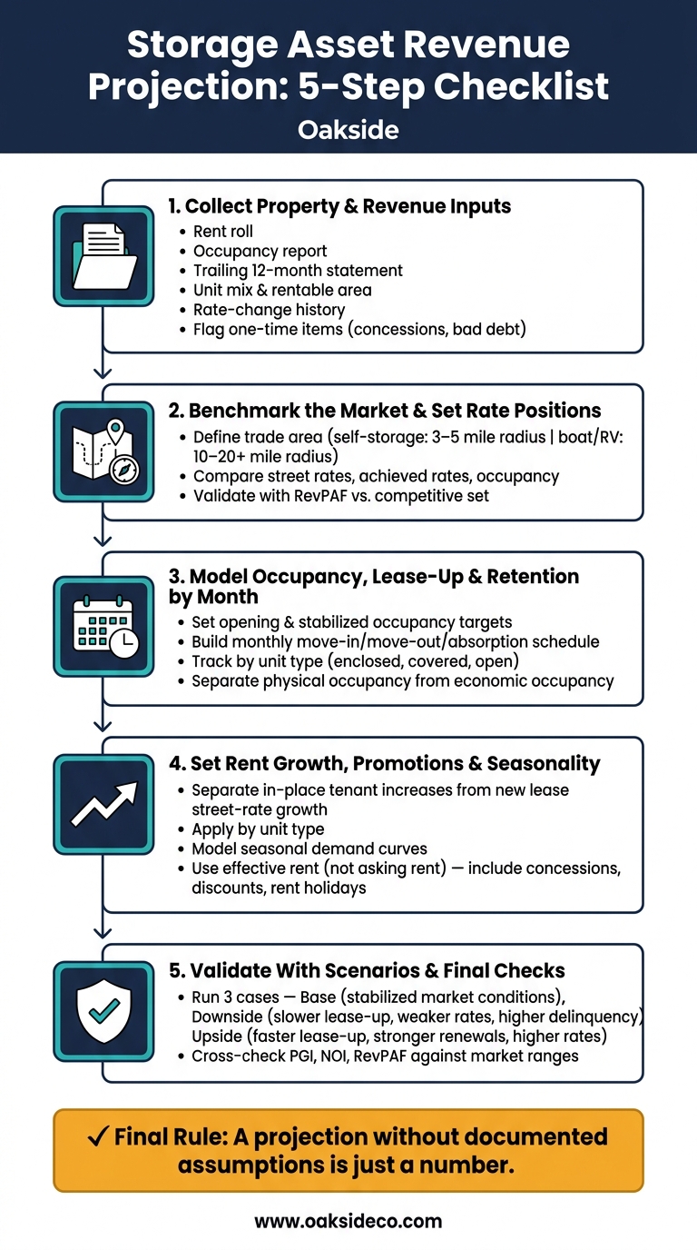
Storage Asset Revenue Projection Checklist: 5-Step Process
Quick comparison
| Area | What I check | Why it matters |
|---|---|---|
| Asset scope | Property type, stage, underwriting goal | Sets the right inputs |
| Property data | Rent roll, T-12, occupancy, unit mix | Builds the starting revenue base |
| Market check | Trade area, comps, street rates, RevPAF | Tests whether rates make sense |
| Monthly demand | Move-ins, move-outs, absorption, stabilization | Shows timing risk |
| Collections | Renewals, delinquency, vacancy lag | Converts occupancy into cash flow |
| Rent plan | Renewal bumps, new lease rates, seasonality, promos | Avoids overstating rent |
| Scenario review | Base, downside, upside | Shows how revenue changes under pressure |
Bottom line: I would not trust a storage revenue projection unless the assumptions are documented, the market check is tight, and the monthly schedule ties back to what the property can actually collect.
sbb-itb-09b4138
1. Collect the Required Property and Revenue Inputs
Start with the records that shape in-place revenue. Gather the rent roll, occupancy reports, trailing income statements, and rate-change history before you build the model. If those records have gaps, one-off promos, or mismatched reporting periods, your revenue forecast can get off track fast.
Reconcile the Rent Roll and Operating Reports
Pull the rent roll, current occupancy report, and trailing 12-month operating statement. Then cross-check them. You want to make sure occupied and vacant spaces, unit mix, rentable area, and ancillary income – wash bays, dump stations, locks, and retail sales – are all included.
These numbers flow straight into physical occupancy, economic occupancy, PGI, and RevPAF.
Flag One-Time Items and Normalize the Data
Compare records from the same reporting period. Log every adjustment in a data log. Then flag one-time concessions, bad debt, and unusual income or expenses so they don’t show up as recurring revenue in the forecast.
Once you’ve reconciled the records, use them to build the rent roll, unit mix, and revenue baseline.
| Required Input | Use in Forecast |
|---|---|
| Rent roll | Establishes occupied units, rates, and unit mix |
| Occupancy report | Sets starting physical and economic occupancy |
| Trailing 12-month operating statement | Identifies true revenue trends and expense baseline |
| Unit mix and rentable area | Drives PGI and RevPAF by unit type |
| Rate-change history | Separates in-place rent trends from new lease rates |
| One-time concessions, bad debt, and extraordinary items | Prevents one-time items from inflating recurring revenue |
| Data log | Records each adjustment and source used |
With the baseline checked, move to market benchmarking and rate positioning. This is a critical step to implement effective pricing strategies that maximize net operating income.
2. Benchmark the Market and Set Rate Positions
Market benchmarking helps you check whether the baseline can support the rent path in your model. The point is simple: make sure the revenue forecast holds up in the market before you move into lease-up and growth assumptions.
Define the Trade Area and Competitive Set
Start by defining the trade area based on asset type, demand drivers, and travel patterns. For self-storage, focus on the local customer base. For boat/RV, use a larger radius that fits how people access storage and how HOA-driven demand shapes the market.
Once the trade area is clear, compare pricing against that market.
Compare Rates and Occupancy
Next, compare projected street rates, achieved rates, and occupancy to the trade-area range. This gives you a way to see whether the forecast is conservative, market-matched, or aggressive before you lock it in.
That matters because it keeps the forecast tied to what the market can actually absorb, not just what the model hopes will happen.
Validate With RevPAF
Use RevPAF as the last check on whether the rate and occupancy plan is producing revenue that makes sense. It shows the combined effect of pricing, occupancy, and unit mix, so you can compare the result with the trade-area range for similar assets.
If RevPAF lands outside that range, go back and revise the rate and occupancy assumptions.
3. Model Occupancy, Lease-Up, and Retention by Month
Turn market demand into monthly occupancy and collections before you layer in rate growth. After you set the rate position, map demand into a monthly occupancy and absorption schedule. That’s the point where benchmarked demand turns into projected revenue.
Set Opening Occupancy and Stabilized Occupancy Target
Use the benchmarked rate position from Section 2 as the anchor for these inputs. Each item below sets either the starting point or the target the model needs to hit:
| Input | What to Record |
|---|---|
| Opening physical occupancy by unit type | Occupied units as a percentage of total units, broken out by unit type or storage format |
| Opening economic occupancy | Collected rent as a percentage of PGI at the start of the projection period |
| Stabilized occupancy target | The physical occupancy percentage the asset is expected to sustain at full performance |
| Timing to stabilization | The number of months from opening occupancy to the stabilized target |
Starting occupancy gives you the baseline. The stabilized target gives you the endpoint. The months in between show the growth path the model needs to follow.
Build a Monthly Lease-Up and Absorption Schedule
Model occupancy month by month. Don’t roll this up into annual averages. Monthly detail is what shows timing risk and cash flow gaps during lease-up.
| Input | What to Record |
|---|---|
| Monthly move-ins | Number of units leased per month by unit type or storage format |
| Monthly move-outs | Number of units vacated per month |
| Net absorption | Move-ins minus move-outs, expressed as units and as a percentage of total inventory |
| Lease-up by unit type or storage format | Separate absorption schedules for each unit category – enclosed, covered, open parking – since demand and fill rates differ by format |
Net absorption is the figure that pushes occupancy forward in the model. Track it by unit type so the schedule reflects actual demand patterns, not one blended average that hides what’s happening.
Account for Retention, Move-Outs, and Economic Occupancy
After the absorption schedule is in place, add turnover and collection assumptions. These inputs turn physical occupancy into the revenue the property is expected to collect:
| Input | What to Record |
|---|---|
| Renewal rate | Percentage of expiring tenants who renew each month |
| Move-out rate | Percentage of occupied units vacating each month |
| Vacancy-to-collections lag | Number of days between a unit becoming vacant and rent collections stopping |
| Delinquency or nonpay occupancy | Percentage of physically occupied units not generating collected rent |
| Economic occupancy formula | Collected rent ÷ PGI, applied monthly throughout the projection period |
Economic occupancy is the figure that links space use to projected cash flow. A unit can be physically occupied and still produce no collected rent if the tenant is delinquent. Model that gap directly. Don’t assume physical occupancy and economic occupancy move together month after month.
Use these occupancy assumptions as the base for rent growth, concessions, and seasonality in the next section.
4. Set Rental Rate Growth, Promotions, and Seasonality Assumptions
Once occupancy and absorption are in place, rate growth becomes the next big revenue driver. Build monthly rent growth by tenant cohort and unit type. Don’t use one blanket growth rate across the entire rent roll.
That shortcut can throw off the model fast.
These inputs should flow into monthly PGI and economic occupancy, not just asking-rate forecasts.
Separate In-Place Tenant Increases from New Lease Rates
Model renewal increases for existing tenants separately from street-rate growth for new leases. Those are not the same thing, and treating them the same can blur what’s happening in the asset.
Annual rent increases for in-place tenants need their own assumptions. Street-rate growth for new leases needs a separate set. Then apply both by unit type, since climate-controlled units, drive-up units, covered RV storage, and uncovered parking each price in their own way.
After you split those tenant cohorts, add monthly demand swings by unit type.
Reflect Seasonal Demand in Monthly Rates and Occupancy
Use trailing 12-month data to build monthly assumptions. Self-storage leasing velocity often tracks summer moving patterns, while boat and RV demand tends to move with seasonal recreation use.
Those shifts affect both occupancy and the market rate you can get. So set separate monthly rate curves for peak periods and slower periods by unit type. Model concessions, discounts, and rent holidays on their own, so effective rent drives revenue, not asking rent.
Use these monthly assumptions as the starting point for scenario testing and final checks. Carry the monthly rate curve into the scenario checks that follow. This ensures your scenario testing accounts for how small shifts in rent or occupancy impact overall returns.
5. Validate the Projection With Scenarios and Final Checks
Once your monthly demand and pricing assumptions are in place, the next step is simple: stress-test the forecast. A projection might look fine on paper, but it also needs to hold up when operating conditions shift.
Run Base, Downside, and Upside Cases
A one-scenario projection won’t tell you how much revenue moves when occupancy, rent growth, concessions, or economic occupancy change. That’s why you should build at least three cases. It lets you see how the model behaves in different conditions instead of betting everything on one straight-line view.
The base case should reflect stabilized market conditions, with occupancy and rent growth lined up with the current rent roll and market benchmarks. The downside case should test slower lease-up, weaker rates, lower renewals, and higher delinquency. The upside case should test faster lease-up, stronger renewals, and modestly higher rates.
For each case, use its own monthly occupancy curve, rate path, and concession schedule. In other words, move the inputs together. If you change only one variable at a time, you can miss how these factors interact in practice.
Cross-Check PGI, NOI, and RevPAF Against Market Ranges
After you run the scenarios, compare the output against market norms and the asset’s unit mix. This is where the model either looks grounded or starts to drift.
Check projected RevPAF against the weighted average of the primary competitive set in the asset’s trade area. If the base case lands well above that range, pause and review the projection before using it for underwriting or pricing.
Then cross-check PGI by applying market street rates by unit type to the unit mix and rentable area. If that doesn’t line up with the model, go back and review the unit mix, rate assumptions, or occupancy inputs.
Conclusion: Final Checklist Before Using the Forecast
Before using the forecast in underwriting or pricing, confirm that:
- Source data is complete and verified – rent roll, historical records, unit mix, and rentable area are reconciled
- Rates are benchmarked to the correct trade area – street rates, achieved rates, and RevPAF are compared against the competitive set
- Occupancy is modeled monthly – with realistic lease-up timing and economic occupancy separated from physical occupancy
- Scenarios are documented and tested – base, downside, and upside cases are reviewed against documented guardrails
A projection without documented assumptions is just a number. This checklist helps make sure the forecast can stand up to underwriting, lender review, and due diligence.
FAQs
What is the difference between physical and economic occupancy?
Physical occupancy is the share of total units that are occupied. Economic occupancy measures the rent you collect against the property’s gross potential revenue.
When there’s a gap between the two, it often points to unpaid rent, delinquencies, or too many concessions. So a property can look full on paper from a physical standpoint, yet still have collection problems that cut into Net Operating Income.
How do I choose the right trade area for self-storage vs. boat/RV?
Start by defining the area your facility can realistically pull customers from.
For self-storage, that usually means a 1 to 3-mile radius in urban areas and up to 5 miles in suburban or rural markets. Boat and RV storage works differently. That customer base often comes from 10 to 15 miles or more.
Next, use GIS mapping to spot access barriers that can shrink that trade area in practice. A river on the map might not look like much, but if there are only a couple of crossings, it can cut demand fast. The same goes for highways, rail lines, or awkward road layouts that make a short trip feel like a hassle.
For self-storage, pay close attention to:
- Population density
- Household formation
- In-migration
For boat and RV storage, look more closely at proximity to recreation, along with local zoning rules or HOA parking restrictions. Those factors often shape demand more than raw population numbers.
Why model revenue projections monthly instead of annually?
Monthly modeling matters because self-storage and boat/RV leases are usually month-to-month. On top of that, demand can swing with the seasons. If you only look at annual projections, you can miss what’s happening on the ground and skew results by 10% to 20%.
Using 12 monthly columns per year gives you a much clearer view. You can apply occupancy and rate assumptions month by month, account for busy stretches like May through September, and follow lease-up speed as the property moves toward stabilization.