Here’s the short answer: penetration rate helps me estimate demand, but it does not tell me if a self-storage project works. I still need to test supply, rents, occupancy, pipeline risk, and lease-up timing before I can say go, wait, or pass.
National household penetration reached 12.6% in 2024, up from about 8.95% in 2005. That shows more households are using storage. But a market can still fail if there is too much space already built, too much new space coming, or weak street rents.
If I’m sizing up a self-storage deal, I focus on four things first:
- Demand: What share of local households rents storage?
- Supply: How many square feet already serve that trade area?
- Rents: Are operators holding prices, or cutting with promos?
- Lease-up: Can a new facility reach 85%–90% occupancy in about 24 to 36 months?
A simple way to think about it:
- Strong penetration + tight occupancy + steady rents = deal may work
- Good penetration + heavy pipeline + weak pricing = slow down
- Weak penetration + soft occupancy + discounting = high risk
I also separate household penetration from square feet per capita. The first is a demand signal. The second is a supply signal. If I mix them up, I can misread the market.
One more point: lenders and buyers do not read this metric the same way. Lenders care about breakeven, debt service, and whether reserves last through lease-up. Buyers care about whether today’s occupancy and rents still hold after new supply hits.
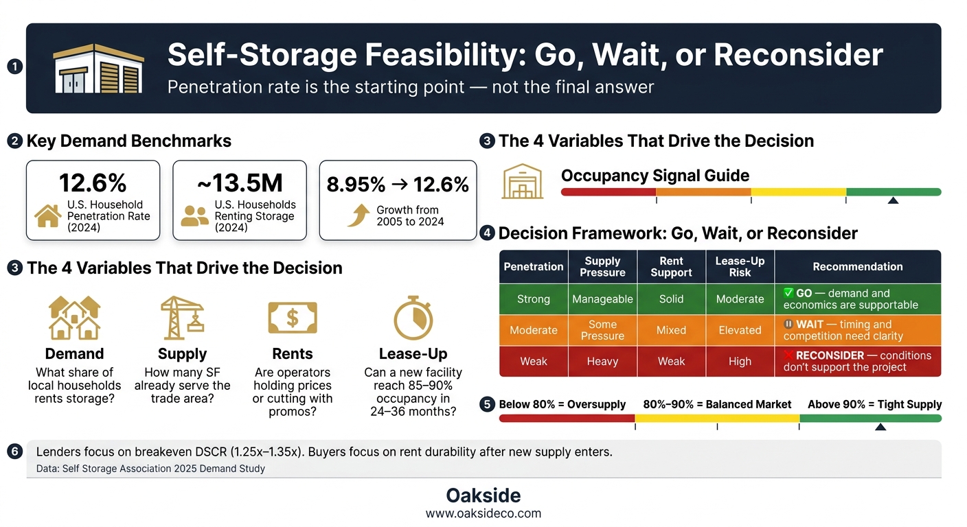
Self-Storage Feasibility: Go, Wait, or Reconsider Decision Matrix
Quick comparison
| Metric | What it shows | What it does not show by itself |
|---|---|---|
| Penetration rate | Share of households renting storage | Whether the market can support more supply |
| SF per capita | How much storage space exists per person | Whether local households are using storage at a high rate |
| Occupancy | How full competing facilities are | Whether current rents are holding without promos |
| Street rents | Current asking price by unit type | Whether operators are collecting those rates after discounts |
| Pipeline | New space that may enter the market | Whether demand will keep pace |
Bottom line: I use penetration as the starting point, not the final answer. The article then turns that demand signal into a plain market test: is there enough unmet demand, at current rent levels, to support a new project or expansion?
sbb-itb-09b4138
Demand Testing: From Household Penetration to Supportable Demand
Selecting the Trade Area and Benchmark Set
Start with the trade area. In day-to-day underwriting, suburban projects usually use a 2- to 3-mile radius, rural sites often stretch to 4 to 5 miles, and dense urban areas may tighten to 1 mile or less.
The point is simple: define the area that sends most of the customers to the facility. That means looking past a clean circle on a map and paying attention to what shapes demand in practice. Highways, rivers, and other barriers can cut off traffic. Nearby clusters of competing facilities can split the same customer base. And both residential pockets and job centers help drive storage use. The end result is the local household base used in the penetration analysis.
After that, compare local penetration with regional and national benchmarks. The Self Storage Association‘s 2025 Demand Study found that U.S. household penetration reached 12.6% in 2024, up from 11.1% in 2022, with nearly 13.5 million households renting storage. Regional rates differ. The South came in at roughly 12.0% in 2026, ahead of the West, Midwest, and Northeast.
These figures give you a reference point. But they don’t decide the deal. The local number does. Once that benchmark set is in place, the next move is turning participation into supportable square footage.
Converting Household Demand into Supportable Square Footage
Once the trade area and participation rate are set, the math is pretty direct. If a trade area has 20,000 households and local behavior points to a 9% participation rate, that works out to about 1,800 participating households. If each renting household uses an average of 90 square feet, supportable demand lands at about 162,000 net rentable square feet (NRSF).
On its own, though, that number is only a starting point.
It has to be tested against the supply already in the market. Analysts line it up against competing facilities in the trade area and look at things like:
- Unit mix
- Actual leased NRSF at stabilization
- Occupancy levels
That demand estimate only starts to matter when it holds up against competing facilities, occupancy, and achieved unit mix.
Variables That Raise or Lower Demand
Four factors have the biggest effect on demand: population growth, renter share, household size, and income. Each one can change both the participation rate and the assumed square footage per customer.
Renter concentration is a big one. Renters move more often, have less storage space at home, and usually use self-storage more than homeowners. Breaking the market out by tenure can sharpen the estimate. For instance, 9,000 renter households at 13% participation and 80 SF each produce about 93,600 NRSF, while 11,000 owner households at 6% participation and 100 SF each add another 66,000 NRSF. Together, that comes to 159,600 NRSF, which can differ quite a bit from one blended market assumption.
Income matters too. Middle-income and upper-middle-income households often own more stuff and have more room in the budget for storage, which can support larger units and longer stays. Markets with high move rates – often tied to job growth, in-migration, or heavy apartment deliveries – also tend to produce more short-term and transitional storage demand. Demographic shifts, including generational aging patterns, can affect both lease-up timing and supportable demand across a 3- to 5-year lease-up horizon.
Those demand drivers flow straight into the supply and rent-support work that comes next.
Supply Review and Rent Support
Existing Inventory, Pipeline, and Occupancy Conditions
Once penetration points to demand, the next step is simple: check whether current and planned supply has already soaked it up.
Start by mapping every competing facility in the trade area. Look at class, age, unit mix, and whether the property offers climate control. Then calculate square feet of existing storage per capita. That local ratio is useful as a first pass, but it shouldn’t drive the whole call. What matters more is the actual competitive set and how full those properties are. A market can seem short on supply on paper and still have weak rent support if nearby operators are cutting rates hard.
That’s where occupancy comes in. Use it to pressure-test the ratio:
- Above 90% usually points to tight supply
- 80%–90% suggests a balanced market
- Below 80% points to oversupply
That’s the first check before testing rent support.
Pipeline risk adds another piece. Self-storage doesn’t have high barriers to entry, so new projects can change the picture fast. Space under construction, projects with permits, and credible planned deals should all be treated as future supply. Add that pipeline to existing inventory to estimate effective future supply at stabilization.
How Rent Support Is Tested
A market can post solid penetration and high occupancy and still struggle to push rents. That’s why rent support needs its own test, based on actual pricing from the competitive set.
The process usually starts with a rate survey matrix. Pull street rates by unit size and type, then convert them into rent per square foot. When the data is there, compare achieved rents – what tenants pay after concessions – to street rates. That helps show the gap between asking rent and collected rent. From there, the analyst can spot the median and upper-quartile rents for key unit types, see which facilities hold premium pricing while staying highly occupied, and measure how hard competitors are leaning on promotions.
Heavy concessions across several properties are a loud signal. If operators keep offering one month free, percentage discounts, or step-up pricing, they’re usually chasing the same limited group of renters, even if penetration looks fine at first glance. Between Q4 2021 and Q3 2023, national street rates fell by as much as 30% from their peak. By January 2024, average rents were down to $84.90 per unit, or 14.4% lower than the prior year.
Here’s what that looks like in practice: if the top competitor is getting $1.75 per sq. ft. on a 10×10 climate-controlled unit at 95% occupancy, and the median is $1.50, a reasonable underwriting range is about $1.55–$1.60 after concessions.
Core Data Inputs and What Each One Tells You
These inputs only mean something when you read them together.
| Core Data Input | What It Indicates | Where It’s Used |
|---|---|---|
| Households | Size of the potential storage-using customer base | Demand testing, penetration calculation, trade area sizing |
| Growth trends | Future expansion of demand and long-term trajectory | Forward demand modeling, pipeline risk assessment |
| Income levels | Ability to pay and appetite for higher-quality product | Rent support analysis, product positioning, underwriting rent assumptions |
| Renter share | Higher likelihood of storage use due to mobility and limited space | Demand uplift factors, penetration adjustments, lease-up expectations |
| Existing inventory | Current supply capacity and product mix | Supply review, penetration metrics, competitive landscape definition |
| Pipeline | Future supply competing for the same demand pool | Effective future supply, saturation risk, lender/buyer risk assessment |
| Occupancy | Current market tightness across competitors | Lease-up outlook, validation of penetration findings |
| Street rates | Market’s visible price ceiling and discount patterns | Rent support testing, underwriting rent assumptions |
| Absorption pace | How quickly new space leases up | Lease-up modeling, lender and investor underwriting |
No single input gives the full picture. The point of the supply and rent review is to see how the pieces line up. Penetration may hint at room in the market. Occupancy may back that up – or poke holes in it. Rent data then shows whether that room turns into cash flow you can actually underwrite. Those findings feed straight into lease-up timing and stabilization risk.
Lease-Up Outlook and Investment Interpretation
From Market Demand to Lease-Up and Stabilization
The demand and supply findings feed straight into the lease-up forecast, stabilization timing, and financing risk. In self-storage, analysts usually express absorption as net rentable square feet (NRSF) leased per month and build that into a month-by-month absorption model.
A common starting point is 2%–3% of NRSF absorbed per month, with adjustments based on local market conditions. From opening to stabilized occupancy, a self-storage project often takes about 24–36 months to lease up. In larger markets, or places with a heavy supply pipeline, that timeline can stretch to 36–48 months. Stabilization usually means the property reaches 85–90% physical occupancy. If several new facilities are set to open within 12–24 months of the subject property, analysts usually slow the base-case absorption rate and push out stabilization to reflect split demand and more promo pressure.
Rate strategy matters too. A newer facility with strong visibility may be able to price at or a bit above market averages, but that only works when the rent support data says it can. If incoming supply is heavy or competitors are leaning on discounts, analysts tend to assume more concessions and a slower step-up from intro rates to market rents.
That lease-up forecast then becomes the backbone for lender stress tests and buyer pricing.
How Lenders Read the Study
Lenders read the feasibility study as a risk file, not a sales story. What they care about most is simple: can the property produce enough cash flow to cover debt service before the interest reserve runs dry?
Their focus usually lands on breakeven occupancy and DSCR. In self-storage, breakeven often falls around 60%–65% economic occupancy, which is the point where NOI covers operating expenses and debt service. From there, lenders want to see a path to a stabilized DSCR of 1.25x–1.35x, based on normalized NOI.
When demand looks thin or the pipeline looks heavy, lenders respond with tighter reserves and lower leverage. They underwrite the downside first. In plain English, they want to know the deal can handle a slower lease-up, pay its debt during lease-up, and still be able to refinance into permanent debt.
How Buyers Read the Study
For buyers, the same work turns into a pricing test and an exit test. They want to know whether today’s occupancy and rental rates will still hold once new supply hits the market.
In a stabilizing or value-add deal, buyers dig into whether in-place rents are durable under current penetration conditions. A property sitting at 95% occupancy may look strong on paper, but if the penetration analysis points to oversupply, that number can be misleading, especially when occupancy depends on heavy discounting. Institutional buyers also study room for rent growth. In underpenetrated markets with strong demographics, they may underwrite meaningful rent growth. In saturated markets, they’re more likely to focus on operating efficiency instead.
They also run downside scenarios tied to new supply. And when penetration data points to lasting saturation risk, they usually move exit cap rate assumptions upward.
Conclusion: Turning Penetration Findings into a Feasibility Decision
Household penetration tells you whether demand is there. Feasibility answers a different question: can that demand support new supply at current rents? That gap matters.
Strong penetration doesn’t cancel out heavy supply or soft rents. On the flip side, moderate penetration can still pencil out when supply is limited and pricing holds up. The final call should be plain: new development, expansion, acquisition, or operations, or no action.
Read the matrix as a quick decision guide, not a full underwriting result.
Decision Framework: Go, Wait, or Reconsider
Use the matrix below to turn the four variables into a clear call:
| Penetration | Supply Pressure | Rent Support | Lease-Up Risk | Recommendation |
|---|---|---|---|---|
| Strong | Manageable | Solid | Moderate | Go – demand and economics are supportable |
| Moderate | Some pressure | Mixed | Elevated | Wait – timing and competition need more clarity |
| Weak | Heavy | Weak | High | Reconsider – current conditions don’t support the project |
That same recommendation can mean different things for debt and equity. Lenders care most about whether the project gets to stabilized occupancy before reserves run dry. Buyers care more about whether today’s pricing still works after stabilization. So this is best used as a screening tool, not full underwriting.
Key Points to Carry into Underwriting
Carry these four points into underwriting:
- Penetration is a demand signal, not a go/no-go answer.
- Supply can shift the answer fast, especially when new deliveries are chasing the same tenant base.
- Rent assumptions need to come from actual comparable street rates, not projections. National advertised self-storage rates declined 1.9% year-over-year in August 2026, which makes aggressive rent growth harder to support.
- Use conservative lease-up assumptions: stabilization around 85%–90% occupancy in roughly 36 months, and longer when supply pressure is high.
The goal of the feasibility study isn’t to justify a project. It’s to decide whether the market supports one.
FAQs
How do I calculate local storage penetration?
Calculate local storage penetration by finding Net Rentable Square Footage (NRSF) per capita in your trade area.
Start by defining the trade area with drive-time analysis. In many urban markets, that usually means a 1- to 3-mile radius. In suburban and rural areas, it can stretch to up to 5 miles.
Next, add up the existing storage supply, measured in NRSF, inside that area. Then divide that total by the trade area population.
Here’s the formula:
NRSF per capita = Total storage supply (NRSF) ÷ Trade area population
If the result is close to 1.68 square feet per person, that can point to an undersupplied market.
What is a good penetration rate for a new project?
There’s no single “good” penetration rate for a new self-storage project. A market’s health comes down to local supply, demand, and growth trends, not one fixed benchmark.
For context, the national average is about 6 square feet per capita. Secondary and tertiary markets often fall in the 3 to 5 square feet per capita range. And in an undersupplied market, that figure may be closer to 1.68 square feet per person within a 3-mile radius.
How should I weigh penetration against new supply?
Use penetration as a sign of actual leased demand. Then stack it up against incoming supply to see if the market can soak up new deliveries fast enough to hold rents and occupancy.
Look closely at pipeline timing over the next 24–36 months. Run base, downside, and upside lease-up scenarios, with the most attention on the downside case. When pipeline pressure builds, lenders usually get more conservative.