

I forecast self-storage occupancy by starting with 24–36 months of records and projecting monthly move-ins, move-outs, and collected rent by unit type. I track both occupied units and square feet because a full small-unit section can hide empty larger units.
Here’s what I include:
- Local demand and competing supply to test whether past leasing trends can continue.
- Seasonal leasing patterns and delivery dates to estimate when each unit type reaches its occupancy target.
- Rent, discounts, and unpaid balances to turn occupied space into a cash forecast - not just billed revenue.
- Downside, base, and upside cases to guide pricing strategies, expansion, refinancing, and hold-or-sell decisions.
Then I compare forecasts with actual results each month. My review triggers might include occupancy missing the forecast by 2 percentage points or collected rent falling 5% below plan.
The goal: <u>a monthly forecast I can check and update</u>, not one occupancy target for the entire property.
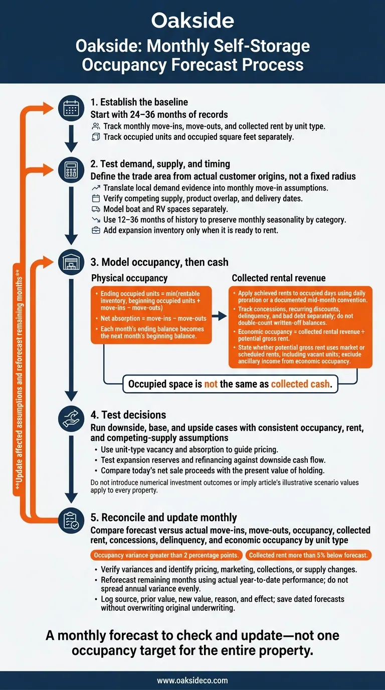
Self-Storage Occupancy Forecasting Workflow
Define the Trade Area and Demand Drivers
Use the historical baseline to check whether local demand supports your forecasted lease-up pace.
Draw the trade area from actual customer origins, not a fixed radius. Test 3-, 5-, and 10-minute drive times for urban properties and 10–20 minutes for suburban and rural properties. Adjust the boundary based on move-in addresses, road access, visibility, traffic, and barriers such as rivers or highways. Separate the primary trade area from the larger area that draws specialty storage customers.
Match local demand indicators with historical move-ins by ZIP code, unit size, and rental reason. Use Census data, Bureau of Labor Statistics employment data, local permits, and college enrollment or military installation data. Population growth is not a rental forecast. Increase projected move-ins only when customer behavior supports that link.
Turn each demand driver into a monthly move-in assumption - not just a market story.
| Demand driver | Supporting data | Forecast effect to test | Risk of overstating demand |
|---|---|---|---|
| Household growth and residential development | Household estimates, permits, completed and occupied homes | Monthly move-ins after residential occupancy begins | Permits may not become occupied homes during the forecast |
| Employment and business activity | Local employment, confirmed hiring, business licenses | Relocation and business-storage move-ins | Workers may live outside the trade area |
| Renter concentration and housing turnover | Rental share, apartment turnover, home sales | Small-unit demand and move-related rentals | Apartments may include storage; low turnover limits demand |
| Military presence | Installation population, relocation and deployment schedules | Timing of move-ins and move-outs | Demand may be concentrated in certain sizes |
| College enrollment | Enrollment, student housing, academic calendars | Seasonal small-unit move-ins and departures | Shared units and price sensitivity can limit rentals |
Map Existing Facilities and New Supply
Survey nearby facilities for rentable square feet, unit mix, quality, climate control, access, advertised rates, promotions, fees, and availability. Confirm key details by phone or in person.
Keep advertised rates separate from achieved rents. If you can't verify achieved rents, label them unknown. Online availability alone does not establish how much inventory is occupied. Use confirmed findings to set rent and absorption assumptions for each unit type.
Measure competing supply by how it affects unit-specific absorption and pricing.
| Project status | Expected delivery | Data to record | Product overlap | Forecast impact |
|---|---|---|---|---|
| Proposed | Uncertain; assess zoning and project progress | Preliminary rentable square feet and unit mix | Likely overlap by size and features | Probability-weight the impact; do not treat delivery as certain |
| Approved | Check permits, financing, and start date | Approved rentable area and configuration | Overlap by product and price segment | Test slower absorption during the likely opening window |
| Under construction | Check observed progress and permits | Confirm planned rentable inventory | Directly overlapping unit types | Model delivery timing and slower subject lease-up |
| Recently delivered | Confirm actual opening date | Completed rentable inventory | Available units matching the subject | Track remaining lease-up inventory and promotions |
Use supply per capita only as a cross-check. It misses product mismatch, access, and vacant inventory. Record each project's source, verification date, delivery confidence, and affected forecast months. Update assumptions when milestones change. Temporary lease-up pressure should not become a permanent occupancy penalty.
Assess Boat and RV Demand Separately
Review local boat and RV registrations, HOA and municipal parking restrictions, nearby marinas and campgrounds, and covered, uncovered, and enclosed inventory. Check whether gate widths, turning space, stall dimensions, and highway access fit the vehicles customers own.
Forecast each space type separately, with its own move-ins, move-outs, rents, and seasonal pattern. Use local leasing history to establish the effects of summer travel and winter storage. Do not use indoor self-storage demand to model boat and RV occupancy without direct customer evidence.
Feed these demand and supply inputs into the monthly model's unit-type absorption assumptions.
Turn your demand and supply assumptions into a monthly operating forecast.
Calculate Absorption by Unit Type
Forecast monthly absorption by unit type, with separate categories for size, climate control, drive-up access, and parking type. For each category, use these formulas:
- Ending occupied units = min(rentable inventory, beginning occupied units + move-ins − move-outs)
- Net absorption = move-ins − move-outs
Multiply occupied units by each unit’s rentable square footage. Then calculate both unit occupancy and square-foot occupancy.
Track delivered units and temporarily unavailable units separately. This keeps repairs, conversions, and closures from distorting vacancy. Add expansion units only when they’re ready to rent.
For existing inventory, use historical move-in, move-out, and renewal patterns. Give new construction and expansions their own delivery dates and lease-up assumptions. Document ownership changes, closures, and promotional periods.
Use this monthly forecast to set seasonality and stabilization assumptions.
Model Seasonality and Stabilization
Use 12–36 months of history to forecast monthly move-ins and move-outs for each category. Tie departures to the occupied tenant base, not total inventory. Keep seasonal patterns intact rather than spreading annual absorption evenly across all months.
Define stabilization as sustained performance against a documented target - not one peak month.
Complete this worksheet for each category. Each month’s ending balance becomes the next month’s beginning balance.
| Forecast month | Unit category | Beginning occupied units | Move-ins | Move-outs | Ending occupied units | Physical occupancy | Occupied square feet | Effective monthly rent | Potential gross rent | Collected rental revenue | Economic occupancy |
|---|---|---|---|---|---|---|---|---|---|---|---|
| Month 1 | Enter category | - | - | - | - | - | - | - | - | - | - |
| Month 2 | Same category | - | - | - | - | - | - | - | - | - | - |
| Month 3 | Same category | - | - | - | - | - | - | - | - | - | - |
Once you’ve forecast physical occupancy, translate it into cash flow.
Calculate Collected Rental Revenue
Apply achieved rents and billing conventions to occupied days. Use daily proration or a documented mid-month convention instead of assigning a full month of revenue to every move-in.
Track concessions, recurring discounts, delinquency, and bad debt separately. Don’t subtract a written-off balance twice if the cash forecast already excluded it.
State whether potential gross rent uses market rents or scheduled rents, including vacant units. Calculate economic occupancy = collected rental revenue ÷ potential gross rent. Keep ancillary income out of this calculation.
Also report collected rental revenue per occupied square foot and per available square foot. Use matching monthly periods and time-weighted occupied area where needed. These figures feed the pricing and hold-sell tests in the next step.
Set Pricing by Unit Type
Use vacancy and absorption by unit type from the monthly occupancy forecast to guide pricing - not just track results. Test rate increases where vacancy is low and concessions where absorption is slow. Model increases for new leases and existing tenants separately. Assess their timing and impact using collected revenue and NOI.
Then test how pricing, leasing pace, and new supply affect occupancy and cash flow.
Test Downside, Base, and Upside Scenarios
Stress-test occupancy, rent, and supply together.
Assumption or result Downside Base Upside Monthly net absorption 4 units 7 units 10 units Competing supply delivered 30,000 square feet 15,000 square feet 0–5,000 square feet Seasonal demand Weak spring/summer uplift Normal seasonal uplift Strong seasonal uplift Achieved rent versus budget -5% 0% +3% Stabilization timing Month 30 Month 22 Month 16 NOI $400,000 $475,000 $535,000 Annual debt service $350,000 $350,000 $350,000 DSCR 1.14x 1.36x 1.53x
Keep rent and occupancy assumptions consistent with the model’s absorption, seasonality, and supply inputs.
Calculate NOI after normalized operating expenses, including management fees, taxes, and insurance, but before capital spending and debt service. Then subtract capital spending and debt service to test liquidity. Defer expansion if slower leasing leaves too little in reserves. Test refinancing against downside NOI, higher interest rates, and the lender’s actual coverage requirement - not just stabilized base-case income.
Compare Holding and Selling
Use the forecast’s expected NOI to compare holding the asset with selling it.
| Decision factor | Hold | Sell |
|---|---|---|
| Remaining lease-up upside | Retain future occupancy and rent growth | Transfer future upside to buyer |
| Capital needs | Fund repairs, expansion, and reserves | Avoid post-closing funding obligations |
| Cash flow | Receive cash after capital spending and debt service | Receive net proceeds at closing |
| Debt obligations | Retain payment and refinancing risk | Repay loan at closing |
| Supply risk | Remain exposed to new deliveries | Supply concerns may affect today’s price |
| Valuation sensitivity | Depends on future NOI and exit cap rate | Depends on current buyer underwriting |
Compare today’s net sale proceeds with the present value of holding. Calculate sale value as forward NOI ÷ cap rate, then subtract selling costs, debt payoff, and closing adjustments. For holding, discount annual after-debt cash flows and future net sale proceeds at the investor’s required return. Stress-test the exit cap rate with a 0.50–1.00 percentage point increase alongside slower NOI growth.
Oakside Co can support occupancy-based underwriting and disposition planning.
Use the forecast as a monthly control model. Reconcile month-end results with the forecast, then update only the assumptions that changed. This check shows whether the original pricing and hold-sell case still holds. Use the same review cycle to reset the remaining forecast months.
Compare Forecasts With Actual Results Monthly
At each month-end, compare projected and actual move-ins, move-outs, occupancy, collected rent, concessions, delinquency, and economic occupancy by unit type. Use reservations and pending move-ins as forward indicators.
Set review triggers ahead of time - for example, an occupancy variance greater than 2 percentage points or collected rent more than 5% below forecast. Verify each variance, then trace it to pricing, marketing, collections, or supply changes.
Keep a short assumption register with the exact source and observation date for each assumption. This record lets you trace the basis for future forecast updates.
| Assumption | Stress cases | Source/date to record | Reason |
|---|---|---|---|
| Trade area | Weaker turnover / stronger household growth | Demographic and housing sources; observation date | Anchor demand locally |
| Supply timing | Earlier / delayed openings | Planning records and site checks; verification date | Time leasing pressure |
| Seasonality | Weaker / stronger peak demand | Operating reports; historical months | Preserve monthly patterns |
| Inventory | Delayed / earlier availability | Rent roll and construction schedule; effective date | Track rentable capacity |
| Stabilization | Later / earlier achievement | Target policy; approval date | Measure lease-up completion |
Reforecast the remaining months using actual year-to-date performance. Do not spread annual variance evenly across the remaining months. Apply revised sensitivity assumptions to each affected unit type, and label changes as temporary, seasonal, or permanent. Then update pricing, stabilization timing, and disposition timing.
Save each dated forecast without overwriting the original underwriting case. For every change, log the source, prior value, new value, reason, and effect.
How do I forecast occupancy without historical data?
When historical data isn’t available, use local market performance to estimate demand. Check nearby occupancy rates, how fast units lease, and rent trends to gauge how quickly the market can fill additional rentals.
Look at household formation and population growth to assess the need for more space. Factor in seasonal shifts, too. Snowbird activity and regional demand for boat and RV storage can help you anticipate changes in occupancy.
How can I estimate move-outs after a rent increase?
Use facility-level data, not broad market averages. Review lease-up rates and move-out patterns around past rent increases over a 24- to 36-month period. This helps separate seasonal shifts from retention changes linked to rent adjustments.
Track physical occupancy alongside economic occupancy - actual revenue collected divided by gross potential revenue. If the gap grows, it may point to higher delinquency or greater reliance on concessions, rather than improved net operating income.
How do I choose a realistic stabilization target?
Assess local market balance using facility-level performance, not anecdotes. Review 24 to 36 months of historical data to separate seasonal swings from deeper demand problems.
Test three scenarios: most likely, downside (weaker demand), and upside (favorable absorption). Account for current market caution by assuming longer lease-up periods and higher vacancy. Base stabilized cash flow on actual collections, not optimistic projections.