
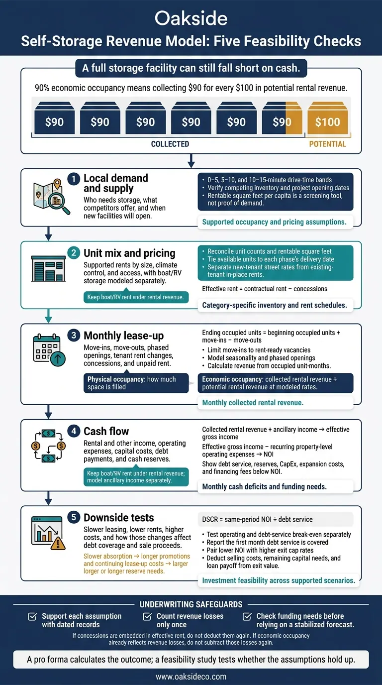
A full storage facility can still fall short on cash. I test collected rent - not just occupied units - to see whether a property can cover expenses and debt payments. For example, 90% economic occupancy means collecting $90 for every $100 in potential rental revenue.
I build the revenue model around five checks:
- Local demand and supply: Who needs storage, what competitors offer, and when new facilities will open.
- Unit mix and pricing: Supported rents by size, climate control, and access, with boat/RV storage modeled separately.
- Monthly lease-up: Move-ins, move-outs, phased openings, tenant rent changes, concessions, and unpaid rent.
- Cash flow: Rental and other income, operating expenses, capital costs, debt payments, and cash reserves.
- Downside tests: Slower leasing, lower rents, higher costs, and how those changes affect debt coverage and sale proceeds.
My rule: <u>support each assumption with dated records</u>, count revenue losses only once, and check funding needs before relying on a stabilized forecast. A pro forma calculates the outcome; a feasibility study tests whether the assumptions hold up.
Self-Storage Revenue Model: Five Feasibility Checks
Trade-Area Demand and Competing Supply
With starting assumptions in place, test whether local demand and supply support the revenue plan. This check sets the bounds for achievable occupancy and pricing - and shapes the occupancy ramp, rent growth, and concessions used later in underwriting.
Use 0–5, 5–10, and 10–15-minute drive-time bands, adjusted for road barriers and access. Review population, household growth, income, renter share, housing turnover, and business activity. The American Community Survey provides demographic and housing data. Compare those findings with facility-level supply in the same trade area. Statewide or metro averages can hide local conditions.
Rentable square feet per capita is a screening tool, not proof of demand. Check it against occupancy, achieved rents, waiting lists, and absorption.
Track proposed, approved, permitted, and under-construction projects separately. Verify each project’s status and expected opening date through planning departments and permit records. Model deliveries in the expected opening month or quarter, and test timing changes for uncertain projects. New inventory opening during lease-up can slow absorption, increase concessions, and put pressure on effective rents - even when existing facilities look well occupied.
Use these demand findings to determine the unit mix the site can support.
Unit Types and Rentable Inventory
Build one inventory schedule that combines size, climate control, and access type to avoid double-counting. Record unit counts, dimensions in feet, net rentable square feet, and starting occupancy by category. Keep boat/RV spaces separate, and reconcile rentable inventory with site constraints before projecting revenue.
For phased projects, tie available units to each phase’s delivery date, not the full buildout. The unit mix determines which rents you can model and how quickly each category can absorb.
Use the table below to record verified inputs. Label missing figures as not available rather than estimating them.
| Inventory group | Unit detail to record | Occupancy input | In-place rent | Street rate | Modeled rent |
|---|---|---|---|---|---|
| Existing local inventory | Size, type, access, count, rentable square feet | Verified market context by category, if available | Achieved rent, if available | Dated advertised rate and concession | Supports subject assumptions |
| Subject existing inventory | Same detail, reconciled to unit records | Actual starting occupancy by category | Rent-roll rate | Current advertised rate | Category-specific forecast |
| Subject proposed phases | Approved layout and rentable inventory by phase | Begins when units become available | Not applicable before opening | Not applicable before opening | Supported rate by category and phase |
| Other proposed supply | Documented unit mix, capacity, status, and delivery date | Unknown before opening | Not applicable before opening | Not applicable before opening | Published pricing, if available |
Once the inventory is defined, test demand by unit type rather than relying on blended occupancy.
Demand Evidence by Unit Type
For an existing asset, review monthly inquiries, reservations, move-ins, move-outs, discounts, and vacancy by size and storage type. Reconcile management reports with rent rolls and unit ledgers. Strong overall occupancy does not validate every size. Strong drive-up occupancy, for example, can hide weak demand for smaller climate-controlled units. For new development, use multiple documented comparables and clearly disclose when category-level operating data is unavailable.
Use this evidence to set move-in, move-out, concession, occupancy, and absorption assumptions by unit type and size.
Underwrite boat/RV storage as a separate product with its own demand curve. Review local vehicle registrations, municipal and HOA parking restrictions, and seasonal demand - not statewide ownership totals alone. Evaluate uncovered, covered, and enclosed spaces separately, including access and maneuverability. Give each type its own rent, seasonal leasing curve, and occupancy assumptions; do not use standard self-storage absorption as a proxy. These inputs feed directly into lease-up timing and revenue projections.
Once demand and unit mix are established, test how pricing and lease-up turn that demand into revenue.
Street Rates, In-Place Rents, and Effective Rents
Test pricing for each supported unit type, then use those rates to calculate lease-up revenue.
Street rates apply to new leases. In-place rents come from existing tenants’ contracts. Effective rent is contractual rent minus concessions; track collection losses and waived fees separately. Back new-tenant pricing with dated local quotes showing unit size, climate control, access, availability, and promotion terms. Save each quote or screenshot, and compare rent per unit and per rentable square foot.
| Rate comparison | Rate basis | Concession treatment | Variance to track |
|---|---|---|---|
| Available new lease | Dated street or web rate for matching units | Record the offer and expiration date | Modeled subject rate vs. supported local rate |
| Existing tenant | Current rent-roll amount | Keep prior discounts separate | In-place rent vs. modeled street rate |
| Effective rental rate | Contractual rent minus concessions | Deduct once; exclude collection losses here | Effective rent vs. contractual rent |
Keep separate pricing schedules for new move-ins and existing tenants. Apply existing-tenant increases only in the scheduled month, based on supported notice periods, tenant tenure, and retention assumptions. Don’t reset those rents to street rates immediately. Assign concessions to the months when they affect cash receipts. If a concession is already included in effective rent, don’t deduct it again.
These assumptions show whether leasing fills units and produces the expected revenue.
Physical vs. Economic Occupancy
Physical occupancy measures how much space is filled. Economic occupancy measures how much potential rental revenue is collected. Use the same inventory and period for both. Calculate economic occupancy by dividing collected rental revenue by potential rental revenue at modeled rates. If the model includes other income or bad debt, define and treat each line item consistently.
| Measure | Formula | Required inputs | Underwriting use |
|---|---|---|---|
| Unit physical occupancy | Occupied units ÷ available units | Rent-ready units and occupied units | Track unit fill |
| Area physical occupancy | Occupied rentable square feet ÷ available rentable square feet | Available and occupied area | Account for size-mix differences |
| Economic occupancy | Collected rental revenue ÷ potential rental revenue at modeled rates | Same-period collections and full available inventory | Measure rental revenue collected |
| Effective rent | Contractual rent minus concessions | Contract rent and concessions | Test pricing after promotions |
Calculate rental revenue from occupied units using tenant rents, then deduct concessions and collection losses. High physical occupancy doesn’t always mean high economic occupancy. Tenants may pay below street rates, receive concessions, or fall behind on payments. Build that revenue gap into the lease-up schedule.
Monthly Lease-Up and Stabilization
Turn pricing and occupancy assumptions into a month-by-month cash flow schedule.
Build the schedule by unit category. Ending occupied units equal beginning occupied units plus move-ins minus move-outs. Net absorption equals move-ins minus move-outs. Calculate revenue from occupied unit-months using the selected rate convention. Show concessions and collection losses separately unless they are already included in effective rent. Identify phased delivery dates, unavailable inventory, and absorption by category. This detailed modeling is a core part of buying and operating self-storage facilities successfully.
| Month | Available units | Beginning occupied | Move-ins | Move-outs | Ending occupied | Month-end occupancy | Effective rent | Concessions | Collection losses | Net rental revenue |
|---|---|---|---|---|---|---|---|---|---|---|
| 1 | A₁ | B₁ | I₁ | O₁ | E₁ = B₁ + I₁ − O₁ | E₁ ÷ A₁ | R₁ | Shown separately or embedded | L₁ | Occupied unit-months × effective rent, less collection losses |
| 2 | A₂ | E₁ | I₂ | O₂ | E₂ = E₁ + I₂ − O₂ | E₂ ÷ A₂ | R₂ | Shown separately or embedded | L₂ | Occupied unit-months × effective rent, less collection losses |
| 3 | A₃ | E₂ | I₃ | O₃ | E₃ = E₂ + I₃ − O₃ | E₃ ÷ A₃ | R₃ | Shown separately or embedded | L₃ | Occupied unit-months × effective rent, less collection losses |
Limit move-ins to rent-ready inventory and available vacancies. Adjust leasing assumptions for seasonality, phased openings, and new supply. Model slower absorption, lower introductory rates, added concessions, or a later stabilization date rather than relying on a straight-line occupancy ramp. Define stabilization as several months of steady physical and economic occupancy. Roll the stabilized monthly schedule into the annual forecast, carrying forward tenant cohorts and recurring turnover.
Rental Revenue and Ancillary Income
Use the monthly lease-up schedule to turn unit-level assumptions into property-level revenue. Calculate monthly gross potential rent (GPR) using the market-tested unit mix and street rates for available inventory. Then use the occupancy ramp to estimate vacancy.
To calculate collected rent, subtract vacancy, concessions, and bad debt from GPR. Reconcile advertised rent with in-place rent, too. Keep boat and RV rent under rental revenue, and model ancillary income separately.
Operating Expenses, NOI, and Cash Flow
State the accounting basis before calculating NOI: effective gross income minus recurring property-level expenses. Include property taxes, insurance, utilities, maintenance, payroll, management, marketing, software, and professional fees.
Test tax reassessment after acquisition or completion. Keep staffing, security, insurance, and other costs that continue during lease-up in the budget. Show reserves, CapEx, expansion costs, financing fees, debt service, owner taxes, and depreciation below the NOI line. Taxes, continuing lease-up costs, and reserve funding can squeeze cash flow before stabilization.
Use an input matrix so reviewers can trace each material assumption to its source.
Illustrative input matrix
Input Unit Source Source date Base Downside Rentable climate-controlled units units Site plan [date] 300 300 Street rent $/unit/month Comparable survey [date] $150 $135 Stabilized economic occupancy % of GPR Comparable lease-up evidence [date] 90% 82% Concession loss % of GPR Rent roll and market review [date] 3% 8% Ancillary income $/month or % of rent T12 and operator evidence [date] $4,000 $2,500 Property taxes $/year Tax assessor [date] $180,000 $210,000 Insurance and utilities $/year Broker quotes [date] $95,000 $115,000 Marketing and payroll $/year Vendor bids and operating budget [date] $140,000 $175,000 Capital expenditures $/year Property-condition report [date] $50,000 $80,000 Debt service $/year Lender term sheet [date] $500,000 $540,000
Treat concession loss as part of economic occupancy - not as another deduction. Use these inputs for break-even, DSCR, and exit sensitivity tests.
Scenarios and Break-Even Tests
Stress the same assumptions together to show how slower lease-up affects cash flow, reserves, and value. Link slower absorption to longer promotions, higher marketing costs, delayed stabilization, and continuing lease-up expenses. Show monthly and annual cash deficits rather than burying them in a stabilized year.
Report the first month debt service is covered, how long reserves must last, and what stabilized value supports.
Directional scenario matrix
Measure Downside Base Upside Lease-up and stabilization Slower; later Supported schedule Faster; earlier Economic occupancy Lower Supported target Higher Rent Lower Market-tested Higher, if supported Concessions Longer or larger Supported offers Shorter or smaller Ancillary income Lower Documented assumptions Higher Operating expenses Higher Underwritten budget Lower, if supported Reserve needs Larger; longer duration Modeled cash deficits Smaller; shorter duration Stabilized NOI Lower Underwritten NOI Higher Exit value Lower NOI; higher cap rate Supported cap rate Higher NOI; supported cap rate
Calculate operating and debt-service break-even separately. Rental income plus ancillary income must first cover operating expenses, then operating expenses plus debt service. Test occupancy and rent together, letting variable expenses change with them.
Calculate monthly and annual DSCR by dividing same-period NOI by debt service. Stabilized coverage can mask lease-up deficits. Development yield equals stabilized NOI divided by total development cost, including financing costs where appropriate.
For exit tests, pair lower NOI with higher exit cap rates. Then deduct selling costs, remaining capital needs, and loan payoff to estimate net sale proceeds.
Once you’ve built the revenue model, check demand, supply, unit mix, pricing, lease-up, and cash flow against market data. The data should support the revenue you’ve underwritten. A range of outcomes tells you more than a single forecast because it shows which assumptions could change the deal.
Underwriting Checklist for Owners and Buyers
Use this final review to check whether your revenue assumptions support the investment:
- Back every material assumption with dated support. Include the source date, geography, unit type, and measurement basis.
- Reconcile unit counts, rentable square feet, and unit-level revenue with property-level totals.
- Count concessions and collection losses only once. Don’t count losses again if economic occupancy already reflects them.
- Link stabilization to your valuation and refinancing assumptions.
- Check that funding covers lease-up deficits and downside reserves.
- Document who approved each assumption and when it needs an update.
- Resolve missing rent-roll details, unverified inventory, and incomplete supply data before closing. If gaps remain, account for that uncertainty in the price, reserves, or loan terms.
Oakside Co’s Advisory Role
Oakside Co helps owners, buyers, and sellers of self-storage and boat/RV assets organize market data, pressure-test underwriting assumptions, and plan transactions and dispositions. Final decisions still depend on verified property and market data.
How can I validate rents before opening?
Validate rents based on what you can collect - not just advertised rates. Compare in-place rents from a current, unit-by-unit rent roll with verified current street rates for each unit type. Note any gaps, reconcile billed rent with cash received, and treat units with delinquencies of 90 days or more as vacant.
Stress-test revenue using at least 12–24 months of monthly history, including concessions. Model seasonality month by month rather than relying on annualized averages.
What if local lease-up data is unavailable?
Use verified facility-level data to assess market demand: occupancy rates, achieved rents versus asking rents, and historical rate trends. If direct data isn’t available, use industry databases that track more than 70,000 facilities to compare achieved rents with market rates and check your assumptions.
For underwriting, stress-test viability with a downside scenario that assumes a 6–12-month lease-up delay and conservative annual rent growth of 3%–8%.
How much cash should I reserve for lease-up?
Set aside enough cash to cover shortfalls during lease-up, which currently takes an average of 36 months to reach stabilization. Stress-test your projections for a 6- to 12-month delay in absorption.
Nolen Masserman, Managing Director at Oakside, warns that debt terms that don’t line up with the project can wipe out equity. Size your debt using a stressed debt service coverage ratio (DSCR) of 1.35x to 1.50x, allowing for potential net operating income shortfalls of 10% to 20%.