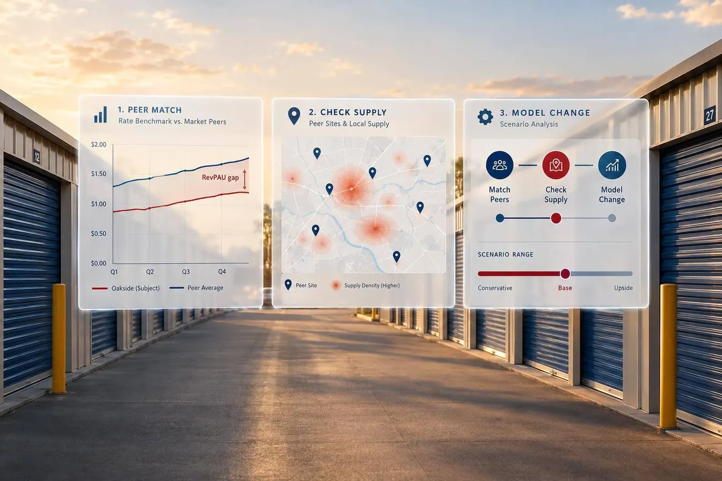


I benchmark self-storage rates against facilities serving the same customers - not market labels. Start with 1-, 3-, and 5-mile rings, check drive times, and compare matching unit sizes, climate control, access, concessions, and fees.
Here’s how I approach each market tier:
- Primary: Check whether convenience supports higher rents despite nearby competition.
- Secondary: Compare housing demand with new storage deliveries and lease-up discounts.
- Tertiary: Test whether limited alternatives support rents across seasons and changes at local employers.
Quick Comparison
| Market tier | Demand to check | Supply to check | Pricing test |
|---|---|---|---|
| Primary | Density, access, job centers | Nearby availability and new openings | Do renters pay more for convenience? |
| Secondary | Housing growth, commute routes | Deliveries and concessions | Can demand absorb new space? |
| Tertiary | Employers, seasonal demand | Direct substitutes and future projects | Do achieved rents hold across seasons? |
For owners, I start with small price tests and track conversion, retention, and collections. For buyers, I use collected revenue, not advertised rents, and phase rent gains into the forecast. <u>A pricing gap is a starting point - not guaranteed income.</u>
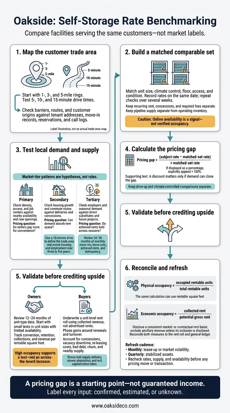
Self-Storage Rate Benchmarking: From Trade Area to Collected Revenue
Treat market-tier patterns as hypotheses, not rules. Test whether local trade-area and supply data support premium, discount, or flat pricing. Use these checks to connect market conditions to rate testing at each facility.
| Market tier | Customer-draw characteristics to verify | Competitive-supply pressures to check | Rate implication |
|---|---|---|---|
| Primary | Dense neighborhoods, short trips, renters, and job centers | Institutional ownership, land constraints, zoning, and high-quality facilities | Convenience and access can support premiums, but nearby availability can limit them |
| Secondary | Suburban growth, new housing, and employment corridors | New deliveries that may outpace household growth | Test pricing gaps against new-facility concessions and lease-up timing |
| Tertiary | Longer drives, concentrated employers, and seasonal demand | Fewer facilities, uneven absorption, and local economic exposure | Verify that occupancy and demand support advertised rates |
Map the Customer Trade Area
After reviewing supply, map where customers actually come from. Start with 1-, 3-, and 5-mile rings, then test 5-, 10-, and 15-minute drive times. Check rivers, bridges, rail lines, limited-access highways, and congested intersections. Test routes at times customers are likely to travel. A nearby facility across a difficult crossing may serve a different renter base.
Check those boundaries against tenant addresses, move-in records, reservations, and call logs. Within each area, review population growth, housing supply, employment growth, and key job centers. Separate residential, commercial, student, military, and seasonal demand where relevant. Record each source’s date so older demographic data doesn’t pass for current information.
Select Nearby Comparable Facilities
Build a set of facilities that compete for the same renters. Choose properties serving the same trade area and offering the same unit types, even if some are farther away. Compare physical features first; use asset class as context. Check condition, access hours, security, visibility, loading access, and management quality. Map ownership separately: several locations with one owner may reflect a single pricing strategy rather than independent market signals.
Use the survey template below for each facility. Record rates on the same date, save source records, and repeat checks over several weeks. Standardize monthly rates by unit size, climate control, floor, and access. Keep promotions and required fees separate. Label estimates clearly, and treat online availability as a signal - not verified occupancy.
| Survey field | Operating-facility entry | Pipeline-project entry |
|---|---|---|
| Facility | Name and address | Project name and address |
| Drive time | Minutes; route and traffic conditions | Minutes; expected access route |
| Asset class and condition | Class, condition, access, security, loading | Proposed specifications; mark unverified details |
| Net rentable square feet | Verified NRSF; mark estimates clearly | Proposed NRSF; source date |
| Unit mix | Sizes and access types | Proposed sizes and access types |
| Climate-control share | Percentage of NRSF; identify denominator | Proposed percentage; identify denominator |
| Vintage | Opening year and major renovations | Expected opening date |
| Ownership profile | Institutional, regional, or independent; common ownership | Owner or developer, if verified |
| Standardized advertised rates | Monthly rates by equivalent unit type | Not available unless published |
| Occupancy or availability | Verified occupancy, available sizes, or waitlists | Not yet operating |
| Concessions | Discount terms, duration, and required fees | Announced opening offers, if any |
| Supply status | Operating; note if recently delivered or in lease-up | Planned, permitted, or under construction |
| Record date and source | Survey date; website, call, or property records | Review date; planning records, permits, or filings |
Keep pipeline supply separate from operating inventory when underwriting current rates. Verify project status through planning records and permits. Track expected delivery dates and overlapping trade areas, then model no-delivery, on-time, and delayed-delivery cases. This modeling serves as a sensitivity analysis to protect equity against shifting market variables.
With the trade area and supply map in hand, assess the subject’s rate position in its primary market. Major metros offer large populations, diverse employment, and a deeper buyer pool. But local demand determines what rents the market can support. A primary-market location doesn’t guarantee higher rents; local comps must support the premium.
Test those market conditions against matched local rates.
Trade Area and Local Supply
Primary markets can support rent premiums, but nearby alternatives and new deliveries can limit them. Review the supply signal before choosing comparables.
Matched Street Rates
Use the framework below to assess the subject’s local position. Enter rates only from dated observations. Keep drive-up and climate-controlled comps separate, and match unit type, access, and condition.
| Comparison | Subject facility | Matched local facilities | Pricing implication |
|---|---|---|---|
| Equivalent unit | Record monthly rent and annualized $/SF | Match size, climate control, floor, and access | Establish the direct premium or discount |
| Customer convenience | Assess loading, visibility, and access hours | Identify meaningful advantages or drawbacks | Test whether a premium has practical support |
| Move-in economics | Separate recurring rent from concessions and required fees | Treat each offer the same way | Distinguish asking rent from net effective cost |
| Availability | Use actual vacant units and leasing results | Record available sizes; verify occupancy where possible | Check whether higher asking rates attract renters |
Pricing Gaps and Underwriting
Calculate whether the subject’s street rate sits above or below matched local comps: (subject rate − matched-set rate) ÷ matched-set rate. A discount matters only if demand can close the gap. Test selected high-demand sizes first instead of increasing rents across every unit type at once. Track conversion, move-ins, realized rent, and occupancy.
Buyers should underwrite a unit-level rent roll, not assume the property can immediately match the highest nearby asking rate. Account for concessions, turnover, bad debt, and lease-up time. Model a partial move toward matched rates, then stress-test new supply and the exit capitalization rate to separate operating upside from rent growth already priced into the deal.
Secondary markets depend on regional demand, not metro size. Housing growth and well-maintained facilities can support premium rents. Low household incomes or heavy new supply can limit them. Use the same comparable-set method as in primary markets, but give more weight to commute patterns, new housing, and the supply pipeline.
Trade Area and Local Supply
Define the trade area by a 10-minute drive, not a fixed radius. Commute routes matter more than distance alone. Review household formation, housing turnover, apartment deliveries, and employment over three to five years. Distinguish demand from established neighborhoods from demand tied to new subdivisions, universities, or military installations.
Track proposed, approved, and under-construction storage separately, recording status, opening date, and NRSF. Measure pipeline space as a percentage of existing inventory. Housing growth won't protect pricing if storage deliveries outpace absorption.
Matched Street Rates
After mapping the trade area and pipeline, compare local street rates at three to five facilities serving the same customer base. Account for facility quality, but don't let it outweigh what local customers will pay.
| Comparison factor | Subject facility | Matched local facilities | Effect on rate positioning |
|---|---|---|---|
| Asset quality and condition | Assess maintenance, visibility, and loading | Separate modern properties from older, basic facilities | Quality alone doesn't justify higher rates |
| Lease-up status | Identify whether the property is stabilized or in lease-up | Flag recent openings and promotional periods | Discounts at new facilities can temporarily limit rates |
| Customer convenience | Evaluate access along residential and commuting routes | Compare facilities serving those same routes | A closer facility may still be a weaker comparable |
| Future supply | Identify exposure by unit type | Record planned openings and competing unit mix | Future competition may affect some sizes more than others |
Pricing Gaps and Underwriting
Use the rate gap between the subject and its comps to distinguish pricing power from temporary lease-up effects. Identify which premiums the market supports and which rate shortfalls reflect weak demand or deferred maintenance.
Tie rent gains to measurable milestones, such as household formation, competing facilities' lease-up progress, or completed improvements. Where deliveries are concentrated, use local evidence to underwrite flat rents, longer promotions, and slower absorption.
Trade Area and Local Supply
Tertiary markets shift the focus from broad population growth to concentrated demand and limited competition.
Pricing power depends on concentrated employers, seasonal demand, and few direct substitutes. Map where customers come from to distinguish the core trade area from renters traveling farther because nearby supply is limited. Distance alone does not prove pricing power.
Review 24–36 months of monthly move-ins, move-outs, achieved rents, and delinquency. Separate seasonal peaks from year-round demand. Few alternatives may support a premium for secure, convenient storage. But cheap land can also make new supply easier to build.
Matched Street Rates
With those demand drivers clear, compare facilities that serve the same renters. Use direct substitutes as pricing anchors and exclude options outside that group. Record availability and promotions alongside posted rents. A newer property or higher advertised rate does not, by itself, prove a premium.
| Comparison factor | Subject facility | Matched local facilities | Pricing implication |
|---|---|---|---|
| Customer reach | Identify core customer origins | Confirm facilities serve the same renters | Exclude distant options that are not substitutes |
| Product match | Record basic features and condition | Match unit size, climate control, and access | Test whether limited alternatives support a premium for basic storage |
| Available inventory | Track vacant units by size | Verify advertised availability | Scarcity may explain a temporary premium |
| Move-in cost | Record rent, concessions, and required fees | Collect identical terms on the same date | Compare effective costs, not headline rents alone |
Pricing Gaps and Underwriting
After comparing direct substitutes, test whether any pricing gap holds up across seasons and the facility’s operating history. Adjust for condition and concessions as part of your self-storage operations. Owners should track conversion, move-outs, and collections when testing targeted rent increases. Buyers should underwrite collected revenue, then separately test employer contraction, off-season vacancy, and new supply.
Customer scarcity and buyer depth are different risks. A facility may have few local substitutes but still attract a narrow pool of acquisition buyers. Back sale assumptions with achieved rents and renewals. Test marketing time and exit cap rates rather than treating temporary strength as permanent growth.
Test Owner Pricing Opportunities
Use the local comp set to check whether the property’s pricing gap holds up. Review 12–24 months of unit-type data, focusing on achieved rents and conversion to see whether nearby rate differences support an increase.
Start with unit sizes that have limited availability. Then track leasing activity, conversion, retention, and revenue per rentable square foot. High occupancy supports a test - not an across-the-board increase.
| Decision rule | Required validation | Underwriting treatment |
|---|---|---|
| Credit below-market pricing only after successful tests | Achieved rent gains without material losses in conversion or retention | Phase in gains based on demonstrated leasing results |
| Address low occupancy before crediting higher advertised rates | Listing accuracy, lead response, conversion, and availability by size | Require an operating plan before crediting upside |
Carry those test results into buyer underwriting. Achievable rent and contract rent are rarely the same.
Set Buyer Rent Assumptions
Turn the owner’s pricing gap into a unit-by-unit rent schedule that accounts for lease terms, concessions, and turnover. Group tenants by move-in date and discount status to estimate what the local market can collect.
Time increases around lease expirations, renewals, and turnover - not an immediate reset at closing. Include vacancy downtime and re-leasing costs. Recognize gains only as tenants renew or units re-lease, accounting for bad debt, churn, and nearby supply.
Physical occupancy = occupied rentable units ÷ total rentable units, or the same calculation using rentable square feet.
Economic occupancy = collected rent ÷ potential gross rent. Use a disclosed, consistent market- or contractual-rent basis. Exclude ancillary revenue unless its inclusion is disclosed. Reconcile both measures to the rent roll and general ledger.
Together, these measures show the difference between occupied space and collected revenue.
Hypothetical underwriting scenarios follow. Each supported assumption requires verification before use.
In-place performance Supported market assumption Downside assumption 10-by-10 units: 88% physical occupancy; $110 average in-place monthly rent Stabilize at 92% occupancy and $120 effective rent over 12 months, supported by signed move-ins at $118–$122 Stabilize at 88% occupancy and $112 effective rent if conversion weakens or a nearby facility adds supply 93% physical occupancy; $145 street rate; $125 collected monthly after concessions Reduce recurring concessions over 18 months and reach $135 effective rent, subject to retention testing and documented concession reductions Maintain $125 effective rent and assume higher churn if discounts cannot be reduced Newly delivered climate-controlled units: 72% occupancy Reach 85% occupancy over 24 months with gradual rate growth and documented traffic support Reach 78% occupancy over 30 months with slower absorption, additional concessions, and no immediate rate growth
Apply Rate Analysis to Transaction Planning
Once the rent assumptions are set, use them in acquisition, refinance, and disposition models. Oakside supports self-storage and boat & RV owners and buyers with property-specific rate analysis for acquisitions, operations, renovations, refinancing, and dispositions.
After underwriting the local comp set, use it as the final check on rate positioning. Compare facilities serving the same customers - not just those closest to the property. Match the product and local trade area. Verify rentable area where possible: nominal 10-by-10 units can differ in usable space.
Check each rate gap against demand, occupancy, concessions, and property condition. Market-tier patterns are starting assumptions, not pricing conclusions. Local facilities set the benchmark.
Label every input as confirmed, estimated, or unknown. Asking rents, online offers, and nearby occupancy data don’t tell you the same thing as achieved revenue.
Date-stamp the benchmark. Update it monthly during lease-up or market volatility, and quarterly for stabilized assets. Before any pricing move or transaction, recheck rates, supply, and availability to keep rate positioning tied to current local data.
How do I benchmark rates when local comparisons are scarce?
Use verified facility-level performance data alongside broader market analytics - not general assumptions. Define your trade area: typically a 1- to 3-mile radius in urban areas or up to 5 miles in suburban and rural markets. Check nearby facilities’ online and on-site pricing regularly.
Track economic occupancy, unit-level turnover, and inquiry volume to confirm performance and spot opportunities for growth.
How long should I test a storage rent increase?
The provided information doesn’t set a fixed testing period. Track facility-level performance, including achieved rents versus asking rents, and compare actual results with your original underwriting. Watch how the increase affects occupancy and revenue. Use those results to check your assumptions and adjust your pricing.
How do I separate pricing upside from acquisition risk?
Use verified facility-level data, not anecdotes. Compare in-place rents with street rates. High occupancy paired with falling street rates may point to weak demand masked by concessions.
Check RevPAF and the gap between physical and economic occupancy, then compare both with nearby facilities. Review demographics and local saturation data to assess whether the submarket can support the location’s growth potential.