

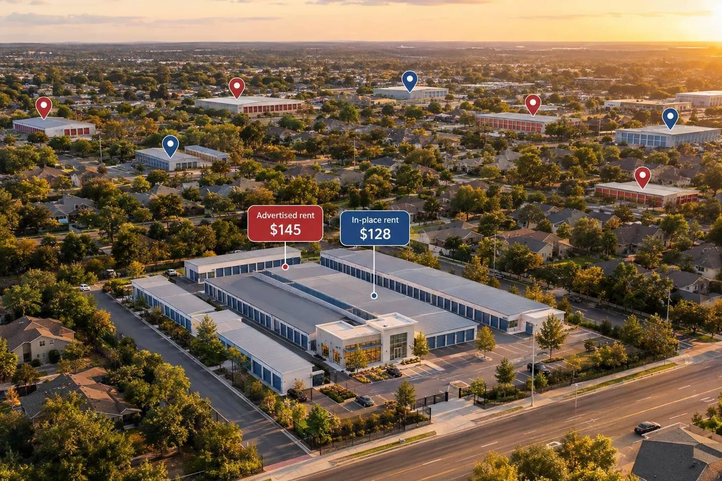
I wouldn’t treat higher self-storage occupancy as proof that rents will recover. The article’s cited research reports advertised rents down 1.6% year over year in July 2026, while tracked REIT revenue grew 0.7% in Q2. My starting point: check local rents, tenant turnover, and nearby supply before assuming income will grow.
For a review through November 11, 2026, I focus on three checks:
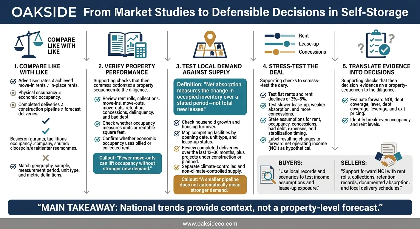
- Compare like with like. Separate advertised rates from rents tenants pay, physical occupancy from rent collections, and completed deliveries from forecasts.
- Test local demand. Check how much occupied space increased - not just how many leases were signed - and map competing facilities by opening date and unit type.
- Put the numbers into the deal. Buyers should test rent declines of 3%–5%, slower lease-up, and more concessions. Sellers should support projected net operating income with rent rolls, collections, retention, and local supply records.
My bottom line: <u>national trends provide context, not a property-level forecast</u>. I use market studies to frame the questions - and property records and trade-area data to test the answers.
Self-Storage Demand Risk: From Market Data to Deal Decisions
Demand Trends and New Supply
National advertised self-storage rates fell 1.1% year over year in February 2026, following a 0.4% decline in January. Rates dropped in 26 of the top 30 metros. Atlanta and Southwest Florida saw larger declines, while Minneapolis and Chicago stayed comparatively stable.
Lower advertised rents signal broad pricing weakness and post-boom normalization, not necessarily a collapse in underlying demand.
New deliveries reached 22.27 million net rentable square feet through Q2 2026, down 27.7% from the same period in 2025.
Slower deliveries may ease future pressure, but delivery figures do not show how much space the market absorbed. That makes the gap between advertised rates and in-place rents the key test for underwriting sensitivity.
Asking Rents vs. In-Place Rents
| Measurement period and sample | Rent finding | Occupancy finding | Interpretation |
|---|---|---|---|
| November–December 2025, Yardi national advertised-rate series | Growth slowed from 0.6% in November to 0.3% in December. | Not reported. | Pricing momentum weakened before 2026. |
| January 2026, Yardi same-store advertised-rate sample | $16.27 per square foot, down 0.2% year over year. | Not reported. | Asking-rate momentum turned slightly negative. |
| February 2026, Yardi national advertised-rate series | Rates fell 1.1% year over year. | Not reported. | New-tenant pricing weakened across most tracked metros. |
| Q2 2026, tracked REIT operating portfolios | In-place rents grew 0.5%. | Occupancy rose 10 basis points. | Higher occupancy did not prove broad demand recovery. |
Yardi tied year-to-date improvement to fewer move-outs, rather than stronger new demand.
In-place rent growth can mask weaker new-lease pricing. Buyers should compare achieved move-in rents, after concessions, with the existing rent roll to identify revenue exposed when current tenants leave. This analysis is a core component of a professional self-storage investment strategy.
The next check is whether occupancy gains reflect real absorption or only better tenant retention.
Occupancy Definitions and Sample Differences
At each property, check whether occupancy measures units or rentable square feet. For economic occupancy, confirm whether the calculation compares billed or collected rent with potential revenue. Vacancy equals 100% minus physical occupancy only when both figures use the same inventory and reporting date. Discounts, delinquency, and free rent can reduce revenue even when units remain occupied.
In January 2026, advertised rates fell 0.5% year over year for non-climate-controlled units but rose 0.2% for climate-controlled units.
Keep those segments separate, distinguish stabilized portfolios from lease-up properties, and compare the same months across years, trade area by trade area, before calling it lasting demand weakness.
Construction and Delivery Exposure by Market
The post-boom slowdown varies by market. Yardi Matrix reported 44.1 million net rentable square feet under construction in July 2026, equal to 2.1% of existing U.S. inventory. Its Q3 2026 forecast projected 52.93 million square feet of deliveries in 2026 and 45.25 million in 2027. Those figures are forecasts, not completed supply.
A smaller pipeline does not automatically mean stronger demand; new deliveries can stay in lease-up and keep rents under pressure when supply outpaces demand.
National advertised rates fell 1.9% year over year in August 2026, even as construction slowed.
Treat any recovery from lower deliveries or stronger housing activity as a projection, not a fact. The gap between pipeline size and actual absorption matters most in underwriting.
Trade-Area Demand and Supply Checks
Net absorption measures the change in occupied inventory over a stated period - not total new leases. State the source’s methodology, geography, sample, and dates. Specify whether it measures units or square feet; construction activity is a separate measure.
Use these local checks to test whether occupancy reflects durable demand or temporary lease-up gains.
| Indicator | Evidence to collect | Lower-risk conditions | Higher-risk conditions |
|---|---|---|---|
| Household growth | Household, population, income, employment, and migration trends | Sustained household formation and growth across several sources | Declining households, weak employment, or growth outside the trade area |
| Housing turnover | Home sales, rental turnover, permits, and multifamily deliveries | Recurring moving-related demand | Low turnover, housing contraction, or distant growth |
| Occupancy | Physical and economic occupancy by unit type and vintage; dates and sample | Stable occupancy at rents the market can support over time | Discount dependence or weak conversion from advertised to in-place rents |
| Net absorption | Change in occupied units or square feet; period and methodology | Positive absorption after deliveries | Flat or negative absorption during nearby lease-up |
| Deliveries | Completed deliveries over the last 12–36 months | Limited additions relative to proven demand | Multiple openings, slow lease-up, or high concessions |
| Construction | Projects under construction or planned, with opening dates and unit mix | Limited near-term supply backed by firm project evidence | Large pipeline, delayed projects moving forward, or concentrated climate-controlled supply |
| Asking rents | Advertised rents by unit size, climate control, access, and promotion; collection date | Comparable rents stable after adjustments | Falling rents, heavy promotions, or lower nearby rents |
Map climate-controlled and non-climate-controlled supply separately to match competing rent tiers and lease-up risk. Match rent units and periods, and distinguish recurring rates from introductory specials. Discount-driven occupancy is weaker evidence than occupied-space growth at effective rents.
No market type is inherently safer; test local demand, access, supply, and pricing. Sellers should use the same tests to support forward NOI and defend pricing, considering how these factors influence self-storage cap rates. These local signals determine how much rent, occupancy, and absorption risk a buyer can underwrite - and whether transaction assumptions are defensible.
Buyer Underwriting: Rent Declines and Lease-Up
Market data matter when they change the underwriting. Use national studies for context, then assess the property using local occupancy, achieved rents, move-ins, move-outs, retention, concessions, bad debt, and net absorption.
Map nearby supply, planned projects, construction, recent deliveries, and expected opening dates within the property’s practical trade area. Translate that space into lease-up pressure and the absorption needed to reach break-even occupancy.
Stress-test lower rents, slower lease-up, weaker absorption, and more concessions. Keep advertised rents separate from achieved move-in rates and in-place rents. Asking rents can hold steady while discounts, waived fees, or lower realized revenue tell a different story.
Label any resulting changes to forward NOI as hypothetical. Show the assumptions for rent, occupancy, concessions, bad debt, expenses, and stabilization timing. Run each scenario through forward NOI, debt coverage, leverage, and exit pricing, and identify break-even occupancy and rent levels.
Seller Preparation: Supporting Forward NOI
Prepare monthly rent rolls and operating statements that show achieved and asking rents, concessions, move-ins, move-outs, retention, delinquency, bad debt, and occupancy by unit type. Reconcile rental revenue to the general ledger and collections.
Explain what drove any improvement: stronger pricing, fewer discounts, a different unit mix, or temporary gains. Support above-market in-place rents with retention records rather than assuming those rents will hold after turnover.
Tie forward NOI assumptions to documented absorption and local delivery schedules. If the property trails nearby facilities after their lease-up periods, examine pricing, management, access, visibility, security, and facility condition. Don’t attribute every shortfall to normalization.
Include a slower-recovery case with flatter rents, extended lease-up, and continued concessions. Research describing stabilization does not establish that every property will recover on schedule. Use those records and scenarios to support forward NOI and the asking price.
Oakside Co's Role in Transaction Preparation
Documented operating performance supports pricing and negotiation. Oakside Co supports operating-data review, transaction preparation, investor outreach, and property disposition. These services help organize and communicate documented performance; they do not eliminate demand, lease-up, financing, or valuation risk.
2025 studies point to post-boom normalization, not a broad recovery. Yardi Matrix reported 0.6% year-over-year advertised-rent growth in November 2025. But Q3 2025 revenue occupancy fell to 90.2%, while weighted-average revenue and NOI also declined.
Conditions still vary sharply by trade area. National construction slowed, but projects already underway can extend lease-up and put pressure on local pricing. Buyers should stress-test flat rents, rent declines of 3% to 5%, and slower absorption by unit type. Sellers should back forward NOI projections with evidence that expected gains can hold up as those local properties open.
Research Limits and Diligence Priorities
These studies use different methods, so diligence matters as much as the headline numbers. Check publication dates, measurement periods, samples, geography, metric definitions, and forecast horizons.
The supplied research does not establish a single national absorption benchmark. Flag figures with missing definitions or materially different methods as unverified or noncomparable, or leave them out. Use current property records, unit-level rent rolls, and trade-area checks of absorption and deliveries.
How far should my self-storage market study extend?
Start with the metropolitan statistical area (MSA), then zoom in on the immediate trade area. Use a consistent 3–5-mile radius or drive-time bands of 0–5, 5–10, and 10–15 minutes. Adjust those boundaries for local road barriers and access limits.
Build your analysis on detailed local data - not broad regional averages. Include 24–36 months of monthly performance data to separate normal seasonal dips from deeper demand problems.
How can I tell whether rent discounts are sustainable?
Look beyond current occupancy. Winter promotions are normal. But if heavy discounts continue through May–August and street rates stay below prior-year peaks, they may point to oversupply, weak demand, or less room to set prices.
Review 24–36 months of data and compare physical occupancy with economic occupancy. Track collected rent - not advertised rates. These measures help separate seasonal dips from lasting demand problems and show whether discounts are trading long-term revenue for occupied units.
When should demand risk change my offer price?
Adjust your offer price when demand signals threaten your revenue or occupancy forecasts. Watch for weakness that lasts beyond seasonal dips, low spring and summer move-ins, discounts that continue through peak season, falling street rates, or high tenant turnover.
Check nearby supply, achieved rents, and occupancy trends. Before finalizing your offer, test how slower lease-up and weaker demand would affect your projections. Revisit your valuation if revenue per available unit or economic occupancy repeatedly falls below your forecast.